Equal-width binning divides a numeric range into intervals with identical widths. For univariate outlier detection, each bin’s count estimates how rare its values are. section 9.6
Extreme values can distort the range: most observations may collapse into an edge bin, intermediate bins may become empty, and moderate outliers may become hidden. section 9.6
Use equal-width binning with these practical cautions:
- Prefer it when rarity within individual numeric features matters; equal-count bins are generally used when searching for rare multivariate combinations. section 9.6
- Treat the number of bins as a consequential parameter rather than assuming a fixed choice. section 9.8
- Inspect the resulting histogram because an extreme value can place ordinary observations together and leave useful distinctions unresolved. section 9.6
Uniform data with extreme values
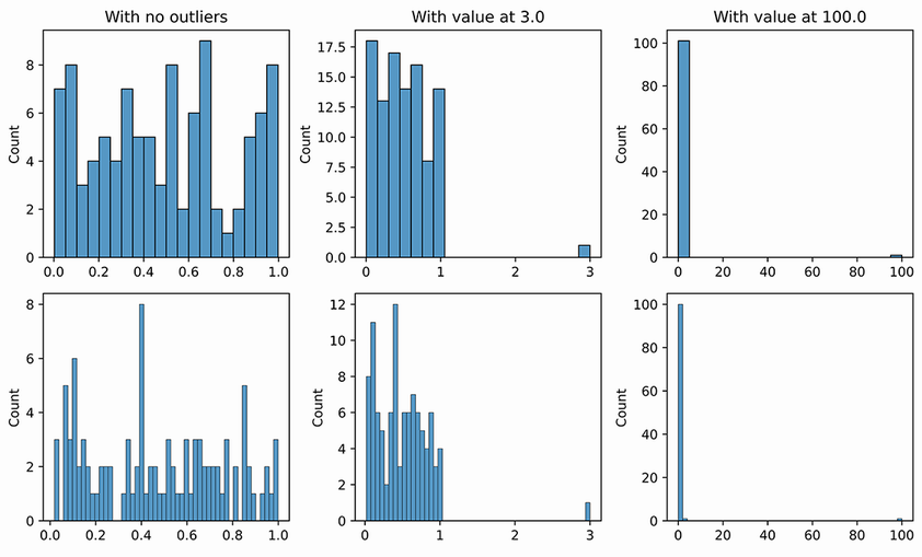
For values distributed between 0.0 and 1.0, adding an outlier at 3.0 can create a sparse bin. Adding another at 100.0 pushes most observations into the leftmost bins; with 20 bins, 3.0 may share an inlier bin, while 50 bins can separate both outliers. section 9.6
Figure 9.1 The effect of the number of bins. In the first row we see where 20 bins are used and in the second row, 50 bins. In each row we see a distribution of uniform data with no outliers (left pane), with a single outlier with value 3.0 (middle pane), and with a second outlier with value 100.0 (right pane). In the top-right pane we see, using 20 bins, the 3.0 value is placed in a bin with inliers. In the bottom-right pane we see, using 50 bins, the 3.0 value is in a separate bin with low count so will be recognized as an outlier.
Compare 20 and 50 bins across clean data and increasingly extreme outliers to see how bin count changes detectability. section 9.6
