The forward-backward algorithm infers latent-state marginal probabilities in a hidden Markov model by combining a forward pass over past observations with a backward pass over future observations. Conditioning on the current state separates the Markov chain into past and future, allowing evidence from the complete sequence through time T. section 7.1.2
Use the following message-passing steps:
- Compute forward messages α recursively from the initial condition and transition and emission probabilities; normalize during each iteration for numerical control. section 7.1.2
- Define the backward message βt(j) = p(xₜ₊₁:T | zₜ = j), then compute it recursively in reverse from t = T, where the terminal future has probability 1. section 7.1.2
- Combine αt(j) and βt(j) to obtain smoothed latent-state marginals γt(j), using observations before and after time t. section 7.1.2
From real-time filtering to smoothing
A forward-only pass can support applications such as handwriting or speech recognition in real time. Adding the backward pass improves state estimates by using the complete observed sequence rather than only data available so far. section 7.1.2
Figure 7.4 Hidden Markov model pseudo-code
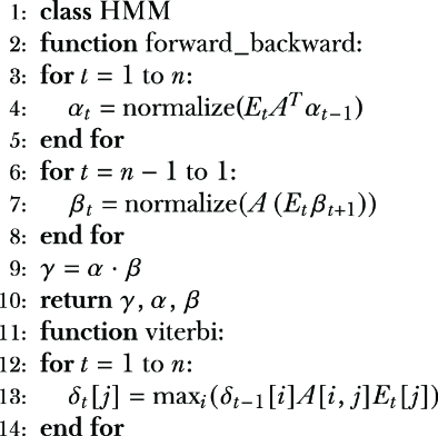
The HMM pseudo-code provides an implementation-level view of the forward_backward routine alongside Viterbi decoding. section 7.1.2
Listing 7.2 Forward–backward HMM algorithm
import numpy as np
from scipy.sparse import coo_matrix
import matplotlib.pyplot as plt

np.random.seed(42)

class HMM():
    def __init__(self, d=3, k=2, n=10000):
        self.d = d     #1
        self.k = k    #2
        self.n = n    #3

        self.A = np.zeros((k,k))   #4
        self.E = np.zeros((k,d))  #5
        self.s = np.zeros(k)      #6

        self.x = np.zeros(self.n)    #7

    def normalize_mat(self, X, dim=1):
        z = np.sum(X, axis=dim)
        Xnorm = X/z.reshape(-1,1)
        return Xnorm

    def normalize_vec(self, v):
        z = sum(v)
        u = v / z
        return u, z

    def init_hmm(self):

        #initialize matrices at random
        self.A = self.normalize_mat(np.random.rand(self.k,self.k))
        self.E = self.normalize_mat(np.random.rand(self.k,self.d))
        self.s, _ = self.normalize_vec(np.random.rand(self.k))

        #generate markov observations
        z = np.random.choice(self.k, size=1, p=self.s)
        self.x[0] = np.random.choice(self.d, size=1, p=self.E[z,:].ravel())
        for i in range(1, self.n):
            z = np.random.choice(self.k, size=1, p=self.A[z,:].ravel())
            self.x[i] = np.random.choice(self.d, size=1,
             p=self.E[z,:].ravel())
        #end for

    def forward_backward(self):

        #construct sparse matrix X of emission indicators
        data = np.ones(self.n)
        row = self.x
        col = np.arange(self.n)
        X = coo_matrix((data, (row, col)), shape=(self.d, self.n))

        M = self.E * X
        At = np.transpose(self.A)
        c = np.zeros(self.n)  #normalization constants
        alpha = np.zeros((self.k, self.n))  #alpha = p(z_t = j | x_{1:T})
        alpha[:,0], c[0] = self.normalize_vec(self.s * M[:,0])
        for t in range(1, self.n):
            alpha[:,t], c[t] = self.normalize_vec(np
             .dot(At, alpha[:,t-1]) * M[:,t])
        #end for

        beta = np.ones((self.k, self.n))
        for t in range(self.n-2, 0, -1):
            beta[:,t] = np.dot(self.A, beta[:,t+1] * M[:,t+1])/c[t+1]
        #end for
        gamma = alpha * beta

        return gamma, alpha, beta, c

    def viterbi(self):

        #construct sparse matrix X of emission indicators
        data = np.ones(self.n)
        row = self.x
        col = np.arange(self.n)
        X = coo_matrix((data, (row, col)), shape=(self.d, self.n))

        #log scale for numerical stability
        s = np.log(self.s)
        A = np.log(self.A)
        M = np.log(self.E * X)

        Z = np.zeros((self.k, self.n))
        Z[:,0] = np.arange(self.k)
        v = s + M[:,0]
        for t in range(1, self.n):
            Av = A + v.reshape(-1,1)
            v = np.max(Av, axis=0)
            idx = np.argmax(Av, axis=0)
            v = v.reshape(-1,1) + M[:,t].reshape(-1,1)
            Z = Z[idx,:]
            Z[:,t] = np.arange(self.k)
        #end for
        llh = np.max(v)
        idx = np.argmax(v)
        z = Z[idx,:]

        return z, llh


if __name__ == "__main__":

    hmm = HMM()
    hmm.init_hmm()

    gamma, alpha, beta, c = hmm.forward_backward()
    z, llh = hmm.viterbi()
The Python listing demonstrates an HMM class with transition, emission, initial-state, normalization, and sparse-observation structures. section 7.1.2
