A hidden Markov model (HMM) represents time-series data with latent discrete states zₜ ∈ {1, …, K}. The states form a Markov chain, while each state emits an observed value xₜ through a state-dependent distribution. section 7.1.2
An HMM is specified by:
- π, the initial state distribution. section 7.1.2
- A, a time-invariant transition matrix with Aᵢⱼ = p(zₜ = j | zₜ₋₁ = i). section 7.1.2
- E, an emission matrix for discrete observations, with Eₖₗ = p(xₜ = l | zₜ = k). section 7.1.2
Inference estimates the unobserved state from emitted observations. The forward quantity αₜ(j) = p(zₜ = j | x₁:ₜ) is computed recursively by summing over predecessor states, multiplying by transition probabilities, and applying the observation update. A forward pass supports real-time inference; a backward pass incorporates observations through time T, producing the forward–backward algorithm. section 7.1.2 section 7.8
Sleep–wake states
A sleep–wake cycle can use K = 2 latent states. The model infers which state generated each observed sequence, while the transition and emission matrices encode state changes and observations. section 7.1.2
Figure 7.3 Hidden Markov model
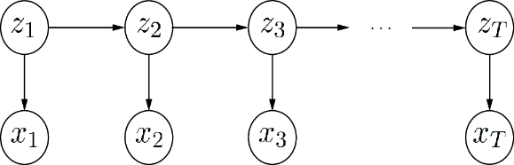
The graphical model makes the latent-state chain, observed emissions, and time-directed dependencies explicit. section 7.1.2
Listing 7.2 Forward–backward HMM algorithm
import numpy as np
from scipy.sparse import coo_matrix
import matplotlib.pyplot as plt

np.random.seed(42)

class HMM():
    def __init__(self, d=3, k=2, n=10000):
        self.d = d     #1
        self.k = k    #2
        self.n = n    #3

        self.A = np.zeros((k,k))   #4
        self.E = np.zeros((k,d))  #5
        self.s = np.zeros(k)      #6

        self.x = np.zeros(self.n)    #7

    def normalize_mat(self, X, dim=1):
        z = np.sum(X, axis=dim)
        Xnorm = X/z.reshape(-1,1)
        return Xnorm

    def normalize_vec(self, v):
        z = sum(v)
        u = v / z
        return u, z

    def init_hmm(self):

        #initialize matrices at random
        self.A = self.normalize_mat(np.random.rand(self.k,self.k))
        self.E = self.normalize_mat(np.random.rand(self.k,self.d))
        self.s, _ = self.normalize_vec(np.random.rand(self.k))

        #generate markov observations
        z = np.random.choice(self.k, size=1, p=self.s)
        self.x[0] = np.random.choice(self.d, size=1, p=self.E[z,:].ravel())
        for i in range(1, self.n):
            z = np.random.choice(self.k, size=1, p=self.A[z,:].ravel())
            self.x[i] = np.random.choice(self.d, size=1,
             p=self.E[z,:].ravel())
        #end for

    def forward_backward(self):

        #construct sparse matrix X of emission indicators
        data = np.ones(self.n)
        row = self.x
        col = np.arange(self.n)
        X = coo_matrix((data, (row, col)), shape=(self.d, self.n))

        M = self.E * X
        At = np.transpose(self.A)
        c = np.zeros(self.n)  #normalization constants
        alpha = np.zeros((self.k, self.n))  #alpha = p(z_t = j | x_{1:T})
        alpha[:,0], c[0] = self.normalize_vec(self.s * M[:,0])
        for t in range(1, self.n):
            alpha[:,t], c[t] = self.normalize_vec(np
             .dot(At, alpha[:,t-1]) * M[:,t])
        #end for

        beta = np.ones((self.k, self.n))
        for t in range(self.n-2, 0, -1):
            beta[:,t] = np.dot(self.A, beta[:,t+1] * M[:,t+1])/c[t+1]
        #end for
        gamma = alpha * beta

        return gamma, alpha, beta, c

    def viterbi(self):

        #construct sparse matrix X of emission indicators
        data = np.ones(self.n)
        row = self.x
        col = np.arange(self.n)
        X = coo_matrix((data, (row, col)), shape=(self.d, self.n))

        #log scale for numerical stability
        s = np.log(self.s)
        A = np.log(self.A)
        M = np.log(self.E * X)

        Z = np.zeros((self.k, self.n))
        Z[:,0] = np.arange(self.k)
        v = s + M[:,0]
        for t in range(1, self.n):
            Av = A + v.reshape(-1,1)
            v = np.max(Av, axis=0)
            idx = np.argmax(Av, axis=0)
            v = v.reshape(-1,1) + M[:,t].reshape(-1,1)
            Z = Z[idx,:]
            Z[:,t] = np.arange(self.k)
        #end for
        llh = np.max(v)
        idx = np.argmax(v)
        z = Z[idx,:]

        return z, llh


if __name__ == "__main__":

    hmm = HMM()
    hmm.init_hmm()

    gamma, alpha, beta, c = hmm.forward_backward()
    z, llh = hmm.viterbi()
The implementation artifact provides a from-scratch forward–backward HMM scaffold with transition, emission, and state-distribution arrays. section 7.1.2
