Gaussian elimination

As explained in Geometry for Programmers

Gauss elimination is a procedure for solving a linear system by systematically eliminating variables from its equations.

Gaussian elimination solves a linear system by changing its equations until the variables appear directly. Scalar multiplication, addition, and row swapping preserve the solution while transforming the coefficient matrix toward triangular or identity form. section 3.6 section 3.6.3

The two-trains system

For Vp − 2Va = 0 and Vp + Va = 450, multiply the second equation by −2, subtract to obtain 3Vp = 900, then continue eliminating until −2Vp = −600 and −2Va = −300. Dividing by the remaining coefficients gives Vp = 300 and Va = 150; substituting these values back verifies both original equations. section 3.6.1

The procedure follows a small set of reversible row operations:

• Scale an equation, multiplying both its coefficients and its free coefficient by the same number. section 3.6.1
• Add or subtract a scaled equation from another to eliminate one variable or coefficient. section 3.6.1
• Swap equations when a needed pivot coefficient is zero; if no suitable coefficient exists, the system may lack that variable or contain dependent equations. section 3.6.2
• Continue until the matrix becomes triangular or, with further normalization, the identity matrix and the right-hand vector becomes the solution. section 3.6.1 section 3.6.2

Figure 3.12 The two-trains problem

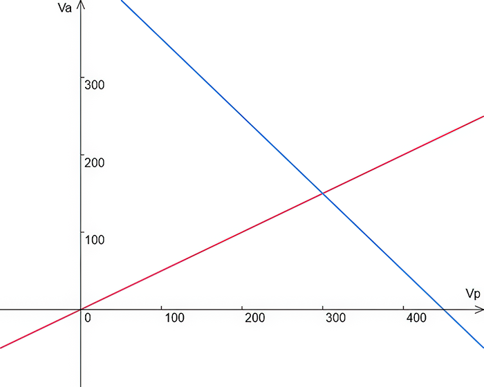
Use the two-trains figure to connect the original pair of equations with their geometric line intersection before following the row operations. section 3.6.1

LU-decomposition uses the closely related idea of factoring a matrix into lower- and upper-triangular matrices. Gaussian elimination, LU-decomposition, and matrix factorization share the same basic approach, while naive implementations have O(N³) theoretical complexity. section 3.6.2 section 3.6.3

How Geometry for Programmers covers it

How deep it goes

Works through a two-variable example, matrix representation, pivot handling, related methods, and naive complexity, without implementation code.

Examples

Uses the two-trains equations, line diagrams, coefficient elimination, matrix reduction, and substitution-based verification.

What it assumes

Assumes familiarity with linear equations and matrices while building the elimination procedure through elementary arithmetic operations.

What you can do after

Apply Gaussian elimination to solve a properly specified linear system and recognize when pivot swapping is necessary.

How it connects

Connects linear systems with row operations, triangular matrices, LU-decomposition, matrix factorization, and inverse matrices.

liveBookmanning.com

Read Geometry for Programmers on liveBook Get the book at manning.com

Related concepts

• scalar multiplicationuses · Scalar multiplication applies a scalar to a mathematical object according to the rules of its algebraic structure, such as scaling a vector or repeated addition of a group element.
• linear systemaddresses · A linear system is a set of linear relationships among variables, commonly expressed as simultaneous equations or a linear transformation, for which superposition applies.
• projective transformationuses · A projective transformation is a mapping of projective-space points represented by homogeneous linear coordinates that preserves incidence but may not preserve parallelism.
• diagonal matrixproduces · A diagonal matrix is a square matrix whose entries outside the main diagonal are zero.

This explainer was generated by Manning's knowledge graph from the text of Geometry for Programmers. The section links point to the parts of the book it draws on.