A geometric cooling schedule lowers simulated annealing’s temperature by multiplying it by a fixed factor α, where 0 < α < 1, at successive cooling steps. Cooling must remain slow enough for the search to stabilize. Larger α values cool more gradually and take longer to reach low temperatures. section 5.2.4
Unlike a linear schedule, geometric cooling approaches zero as the iteration count grows without requiring a predetermined maximum number of iterations. Its gradual decay can produce consistent, timely solutions, but the best factor still depends on the problem. section 5.2.4 section 5.6
Apply the schedule by:
- Choose an initial temperature, a cooling factor, and the number of iterations performed at each temperature. section 5.3
- Run the simulated annealing search, accepting improving solutions and sometimes accepting worsening solutions according to temperature-dependent probability. section 5.3
- After each temperature interval, multiply the current temperature by α and continue until the stopping condition is reached. section 5.2.4
- Tune α experimentally: values around 0.7–0.95 are commonly used, with higher values producing slower cooling. section 5.2.4 section 5.6
Hand calculation
For f(x) = (x − 6)^2, start with T₀ = 5, two iterations per temperature, and α = 0.85. After the first two iterations, update the temperature to T₁ = 5 × 0.85 = 4.25. The search then uses 4.25 for the next temperature interval while generating and evaluating new candidates. section 5.3
Routing application
For a delivery semi-truck traveling between selected Walmart Supercenters, simulated annealing reduced an initial 593.88-kilometer route to a 227.17-kilometer route. Geometric cooling was identified as a possible source of consistent, timely, higher-quality solutions, subject to tuning. section 5.6
Figure 5.8 Different SA cooling schedules
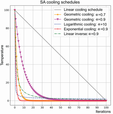
Compare the different simulated annealing cooling curves and see how geometric cooling declines more gradually. section 5.2.4
