Hierarchical risk parity

Hierarchical risk parity (HRP) constructs a risk-parity portfolio without manually specifying an asset tree. It learns a hierarchy from asset correlations, groups related assets, reorders the covariance structure around those groups, and assigns weights by repeatedly splitting clusters. The aim is a diversified allocation in which high-volatility holdings do not quietly dominate portfolio risk. section 11.2.4 section 11.4

Start with return data, an annualized covariance matrix, and a correlation matrix. Convert correlations to pairwise distances using Dᵢⱼ = √((1 − Rᵢⱼ)/2): assets with higher correlation have smaller distances. Then compare each asset’s full distance profile to every other asset through a second Euclidean-distance matrix. Clustering this matrix joins the closest assets into progressively larger groups. section 11.2.4

import itertools

tickers = ['VV', 'VB', 'AGG', 'VEA', 'BNDX', 'VWO', 'EMB', 'DJP']           
rets = yf.download(tickers, start='2014-01-01', end='2021-12-31')['Adj Close']
rets = rets.pct_change().dropna(axis=0, how='any')[tickers]
cov, corr = rets.cov() * 252, rets.corr()

dist = ((1 - corr) / 2.) ** .5

d_bar = dist * 0
for i, j in itertools.permutations(dist.columns, 2):
    d_bar[i][j] = np.linalg.norm(dist[i] - dist[j])

This implementation derives correlation and covariance estimates for eight ETFs, then computes both the direct correlation-distance matrix and the distance-profile matrix used for clustering. section 11.2.4

The cluster linkage determines an ordering of the assets. Reordering the correlation matrix by that ordering places similar assets near one another, making the cluster structure visible as blocks in a heatmap. This ordered list is also the input to recursive bisection. section 11.2.4

Figure 11.6 Visual depiction of the cluster-splitting process, resulting in reordered assets

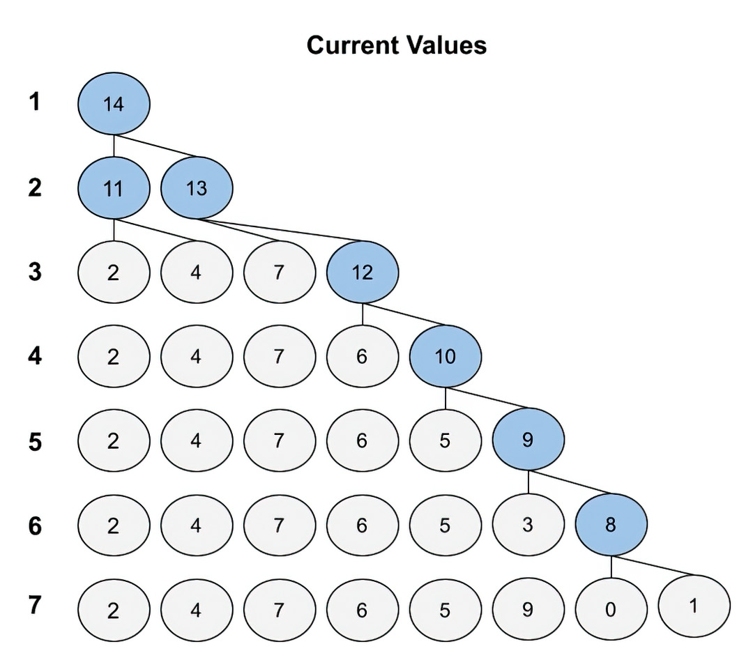
The cluster-splitting diagram shows how the hierarchy produces an ordered asset list before weights are assigned. section 11.2.4

Recursive bisection begins with weight 1 for every ordered asset and repeatedly divides each non-singleton cluster into left and right halves. For each half, compute cluster variance using inverse-variance weights within its covariance submatrix. If left and right variances are Vₗ and Vᵣ, set α = Vₗ/(Vₗ + Vᵣ), multiply left-side weights by 1 − α, and right-side weights by α. Continue until every cluster contains one asset. section 11.2.4

A practical HRP workflow is:

• Estimate returns, covariance, and correlations for the candidate assets. section 11.2.4
• Transform correlations into distances and hierarchically cluster the assets. section 11.2.4
• Reorder assets from the linkage structure, then recursively bisect the ordered clusters. section 11.2.4
• Calculate portfolio variance and asset risk contributions to inspect the resulting allocation. section 11.2.4

HRP is an alternative to calculating risk-parity weights through convex optimization with target asset contributions. Like other risk-parity approaches, it targets diversification, but a portfolio designed around balanced risk may require leverage to reach expected returns comparable to traditional portfolios; obtaining leverage carries costs. section 11.4