An income distribution shows how total income is divided among the members of a population. It can be nearly equal, with similar incomes for everyone, or concentrated, with a small group receiving much of the total. In NBA salary analysis, the population is players and the income values are salaries; comparing distributions asks whether a team’s pay is spread broadly or concentrated in a few highly paid players. section 12.0 section 12.1
The Gini coefficient summarizes inequality on a 0-to-1 scale: 0 means perfect equality and 1 means perfect inequality. Higher values mean a more dispersed distribution. It is a relative measure, though, so matching Gini values do not imply matching income levels, living standards, or distribution shapes. section 12.1 section 12.5
Read a distribution with complementary tools:
- Use the Gini coefficient to compare the overall concentration of income across populations or seasons. section 12.1
- Use a Lorenz curve to plot cumulative income or wealth distribution against the share of individuals; compare its inequality curve with the diagonal for perfect equality. section 12.6
- Use t-tests and effect-size tests when comparing Gini coefficients between groups, such as championship and non-championship teams. section 12.7.2 section 13.9.2
Same inequality, different income levels
Five people earning $50 and five earning $100 produce a Gini coefficient of 0.17. Replacing those incomes with $150 and $300 still produces 0.17: incomes rose, but the same half of the population receives two-thirds of total income. By contrast, nine people earning $10 while one earns $100 produces a much higher Gini, about 0.43. section 12.5
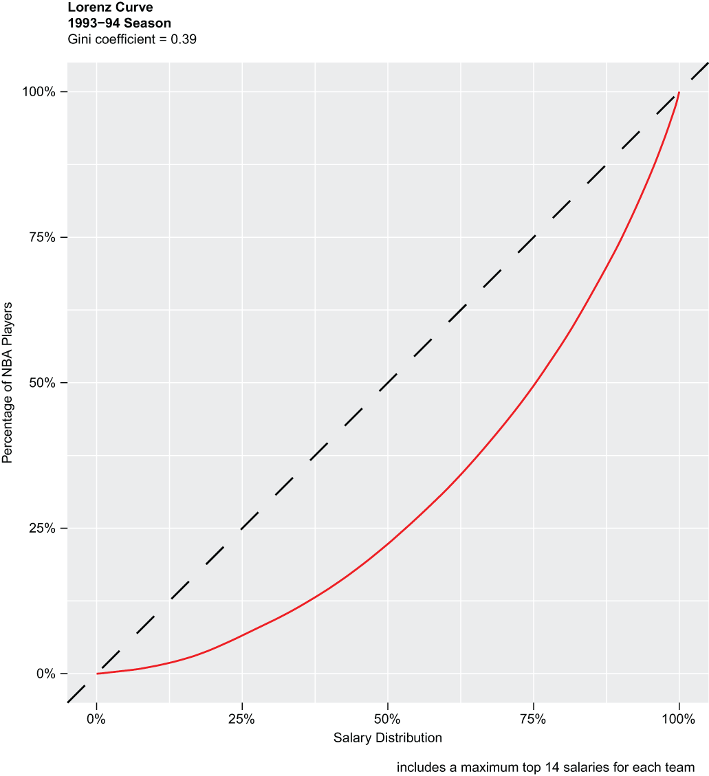
This Lorenz curve visualizes the 1993–94 NBA salary distribution, whose Gini coefficient of 0.39 was the lowest in the data set. section 12.6
Applied to NBA teams from 1991–2018, more unequal salary distributions aligned with stronger results rather than the initial expectation of greater equality. Championship teams averaged a Gini coefficient of 0.53 versus 0.48 for other teams, and teams at or above 0.40 won at least 54% of regular-season games on average. These comparisons describe an association in this data, while the Gini alone still conceals important distribution details. section 12.7.2 section 12.9 section 12.1
The same approach can measure distributions beyond salaries. Computing annual Gini coefficients for player win shares shifts the question from how compensation is allocated to how player productivity is distributed. section 13.0 section 13.4
