Imagine measuring atmospheric CO₂ each year. A reading gives you evidence about the underlying concentration, but measurement noise means the reading and the true level need not match exactly. That underlying, unobserved value is a latent state. section 9.2
A state-space model describes how the latent state changes over time and how it produces observations. A filter uses both relationships in a repeating cycle: predict the next state, then revise that prediction when a new reading arrives. A Bayesian filter keeps this belief as a probability distribution, so estimates carry uncertainty. section 9.2 section 9.3 section 9.4
What belongs in the state depends on what you need to predict:
- A random-walk model uses one number: the current CO₂ level. It can respond to new readings, but its mean forecasts stay flat over multiple years because it does not represent a persistent trend. section 9.11 section 9.10
- To represent a trend, use a latent state vector with two components: CO₂ level and its yearly change, or slope. The next level depends on both; the slope can also change from year to year. section 9.12
- The observation model relates the measured CO₂ reading to the level component, with observation noise. The slope need not be measured directly to help predict future levels. section 9.12
Figure 9.3 A diagram of a state space model, which includes an unknown latent space 𝑥ᵢ that evolves over time, and the observation model, which describes the relationship between the latent state and observed data 𝑦ᵢ at each time step.
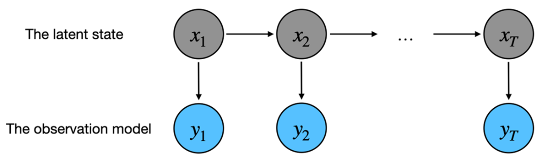
Follow each unobserved state across time, then compare it with the observation linked to that time step. The diagram makes the distinction between a changing state and its measured data visible. section 9.2
Updating a CO₂ estimate
Suppose a filter has estimated this year's underlying CO₂ level. Before seeing next year's reading, it predicts the next state using the transition model. Once the reading arrives, it updates that prediction through the observation model. In the Gaussian implementation, means and variances track both the prediction and its uncertainty. section 9.3 section 9.8
