A latent variable is unobserved and must be inferred from observed data through a probabilistic model. In a hidden Markov model (HMM), discrete latent states zₜ generate observations xₜ through an emission matrix, while a transition matrix models movement between states. section 7.1.2
For an HMM, infer the posterior state probability p(zₜ = j | x₁:ₜ). The forward algorithm computes these marginals recursively with an initial state distribution, transition probabilities, and emission probabilities; the forward–backward algorithm adds future observations through a backward pass. section 7.1.2
Figure 7.3 Hidden Markov model
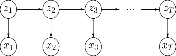
Use the graphical model to trace how latent states connect across time and emit observed data. section 7.1.2
Listing 7.2 Forward–backward HMM algorithm
import numpy as np
from scipy.sparse import coo_matrix
import matplotlib.pyplot as plt

np.random.seed(42)

class HMM():
    def __init__(self, d=3, k=2, n=10000):
        self.d = d     #1
        self.k = k    #2
        self.n = n    #3

        self.A = np.zeros((k,k))   #4
        self.E = np.zeros((k,d))  #5
        self.s = np.zeros(k)      #6

        self.x = np.zeros(self.n)    #7

    def normalize_mat(self, X, dim=1):
        z = np.sum(X, axis=dim)
        Xnorm = X/z.reshape(-1,1)
        return Xnorm

    def normalize_vec(self, v):
        z = sum(v)
        u = v / z
        return u, z

    def init_hmm(self):

        #initialize matrices at random
        self.A = self.normalize_mat(np.random.rand(self.k,self.k))
        self.E = self.normalize_mat(np.random.rand(self.k,self.d))
        self.s, _ = self.normalize_vec(np.random.rand(self.k))

        #generate markov observations
        z = np.random.choice(self.k, size=1, p=self.s)
        self.x[0] = np.random.choice(self.d, size=1, p=self.E[z,:].ravel())
        for i in range(1, self.n):
            z = np.random.choice(self.k, size=1, p=self.A[z,:].ravel())
            self.x[i] = np.random.choice(self.d, size=1,
             p=self.E[z,:].ravel())
        #end for

    def forward_backward(self):

        #construct sparse matrix X of emission indicators
        data = np.ones(self.n)
        row = self.x
        col = np.arange(self.n)
        X = coo_matrix((data, (row, col)), shape=(self.d, self.n))

        M = self.E * X
        At = np.transpose(self.A)
        c = np.zeros(self.n)  #normalization constants
        alpha = np.zeros((self.k, self.n))  #alpha = p(z_t = j | x_{1:T})
        alpha[:,0], c[0] = self.normalize_vec(self.s * M[:,0])
        for t in range(1, self.n):
            alpha[:,t], c[t] = self.normalize_vec(np
             .dot(At, alpha[:,t-1]) * M[:,t])
        #end for

        beta = np.ones((self.k, self.n))
        for t in range(self.n-2, 0, -1):
            beta[:,t] = np.dot(self.A, beta[:,t+1] * M[:,t+1])/c[t+1]
        #end for
        gamma = alpha * beta

        return gamma, alpha, beta, c

    def viterbi(self):

        #construct sparse matrix X of emission indicators
        data = np.ones(self.n)
        row = self.x
        col = np.arange(self.n)
        X = coo_matrix((data, (row, col)), shape=(self.d, self.n))

        #log scale for numerical stability
        s = np.log(self.s)
        A = np.log(self.A)
        M = np.log(self.E * X)

        Z = np.zeros((self.k, self.n))
        Z[:,0] = np.arange(self.k)
        v = s + M[:,0]
        for t in range(1, self.n):
            Av = A + v.reshape(-1,1)
            v = np.max(Av, axis=0)
            idx = np.argmax(Av, axis=0)
            v = v.reshape(-1,1) + M[:,t].reshape(-1,1)
            Z = Z[idx,:]
            Z[:,t] = np.arange(self.k)
        #end for
        llh = np.max(v)
        idx = np.argmax(v)
        z = Z[idx,:]

        return z, llh


if __name__ == "__main__":

    hmm = HMM()
    hmm.init_hmm()

    gamma, alpha, beta, c = hmm.forward_backward()
    z, llh = hmm.viterbi()
Use the Python listing to implement HMM parameters, normalization, and forward–backward inference rather than treating latent-state estimation as a black box. section 7.1.2
Concrete uses and practice include:
- Model a sleep–wake cycle with two latent states, or apply the same structure to stock prediction and DNA sequencing. section 7.1.2
- Compare inferred latent states z with ground-truth states in the forward–backward HMM exercise. section 7.7


