Likelihood measures how well a parameterized probability model accounts for observed data. With data X fixed and parameters θ varied, the likelihood p(X|θ) assigns each candidate θ a score from the chosen model family. Parameter estimation seeks values that make this score large. section 6.6.1 section 13.1
For independent training instances, the overall likelihood is the product p(X|θ) = ∏ᵢ p(x⁽ⁱ⁾|θ). Each factor is the probability density supplied by the model family. A Gaussian model, for example, uses a Gaussian density whose mean and covariance are the parameters to estimate. section 6.6.1 section 13.1
A useful geometric interpretation is overlap: a well-fitting likelihood generates a sample cloud that largely overlaps the training data. For a Gaussian, its mean should lie near a dense region of points, while its covariance should form an ellipse that tightly contains many observations. section 13.1
Likelihood participates in several estimation objectives:
- Maximum likelihood estimation (MLE) chooses θ using only p(X|θ). section 13.11
- Maximum a posteriori (MAP) estimation maximizes p(X|θ)p(θ), combining the likelihood with a prior that can favor smaller parameter magnitudes. section 6.6.3
- As the data set grows, the likelihood has increasing influence on the posterior, while a fixed prior matters less. section 6.6.3 section 13.3
Gaussian negative log-likelihood
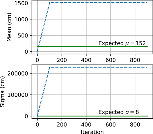
Likelihood maximization can be implemented as minimization of negative log-likelihood. For Gaussian data, a PyTorch loss computes terms involving the sample count, log variance, and squared distance from the mean; gradient descent then updates μ and σ. Starting MLE far from expected values may cause parameters to grow very large, whereas MAP adds squared-parameter regularization through the prior. section 6.8.2 section 6.8.2
Likelihood also describes conditional data generation in mixture models. In a Gaussian mixture, p(x|k) is the likelihood of data value x after class or component k is selected; multiplying it by the component probability p(k) yields the joint probability p(x,k). section 6.9.2
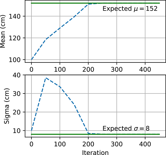
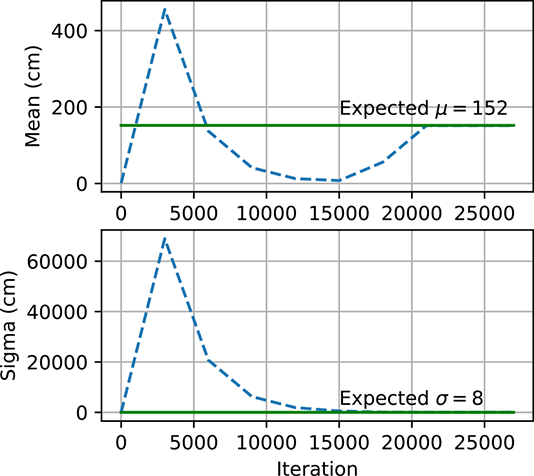
Figure 6.5 Gaussian parameter estimation using maximum likelihood estimate and maximum a posteriori estimation. In figure 6.5a, the MLE explodes because μ and σ are initialized far from μexpected and σexpected. However, the MLE converges in figure 6.5b because μ and σ are initialized closed to μexpected and σexpected. Figure 6.5c shows how, for MAP, μ and σ are able to converge to μ.expected and σexpected even though they are initialized far away.
|
(a) MLE explodes: μinit = 1, σinit = 1. |
|
(b) MLE converges: μinit = 100, σinit = 10. |
|
(c) MAP converges: μinit = 1, σinit = 1. |
Compare how initialization affects Gaussian MLE and how adding a prior in MAP regularizes the optimization. section 6.8.2




