Linear approximation replaces a curve or scattered measurements with a line that captures local behavior or an overall trend. Geometrically, a line segment joining two points approximates a function across an interval; as the interval shrinks, it approaches the tangent line at a point. section 5.1.1
Two practical uses stand out:
- Use the slope of a secant line as an average growth measure across an interval. This gives a simple line-based picture of how a function changes. section 5.1.1
- Use the tangent-line idea to describe growth at a specific point, including matching values and growth rates when joining functions smoothly. section 5.1.1
- Fit a degree-one polynomial to data with least squares. The resulting line summarizes an assumed linear trend rather than explaining every fluctuation. section 6.2.3
Rowing times as a linear trend
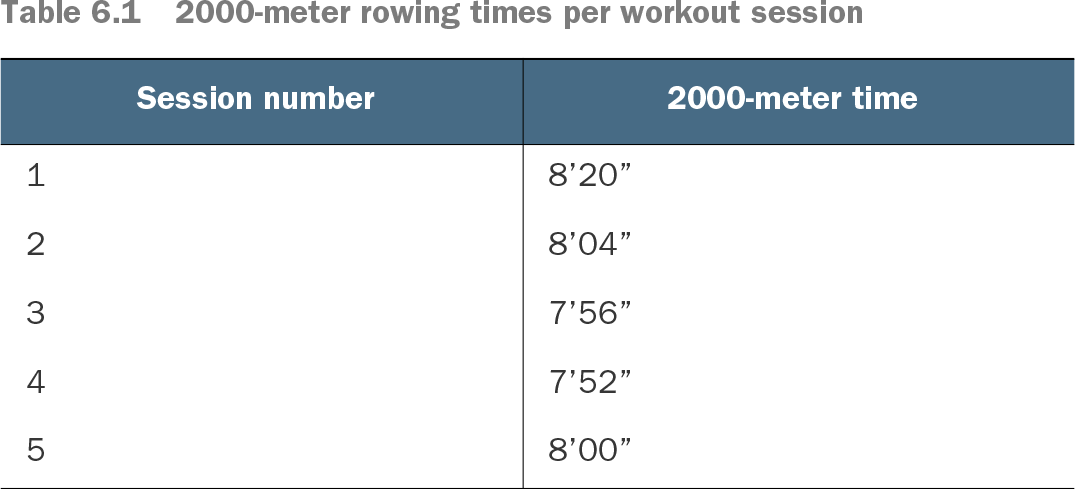
Five 2000-meter rowing times are converted to minutes and paired with session numbers. With polynomial degree M = 1, Python and SymPy construct the least-squares matrix, build the right-side vector from the measured values, solve for a0 and a1, and obtain the approximating line. The plotted trend is useful for visualizing progress, although extrapolating it can produce an implausible prediction. section 6.2.3
Table 6.1 2000-meter rowing times per workout session (view table figure)
Inspect the five-session rowing dataset used to motivate the linear fit. section 6.2.3
Listing 6.1 Computing the approximating polynomial
LS = Matrix([[sum([xs[i]**(row + column)         #1
    for i in range(N)])                          #1
        for column in range(M+1)]                #1
            for row in range(M+1)])              #1

B = Matrix([sum([ys[i]*(xs[i]**row)              #2
    for i in range(N)])                          #2
        for row in range(M+1)])                  #2

a0, a1 = symbols('a0 a1')
Pol = Matrix([a0, a1])                           #3

solution = solve(LS*Pol - B, (a0, a1))           #4
a = [value for key, value in solution.items()]   #5
Follow the complete SymPy listing that constructs the least-squares system and solves for the two coefficients of the line. section 6.2.3