A linear system is a collection of linear equations that must all hold at once. Each variable appears only to the first power, multiplied by a coefficient. A solution assigns values that satisfy every equation; depending on the equations, there may be one solution, infinitely many, or none. In practical work, an approximate answer can sometimes still be useful even when no exact common solution exists. section 3.1 section 3.11
Geometry makes the idea easier to see. In two variables, each equation is a line, so solving two equations means finding their intersection. In three variables, equations become planes. More generally, an equation in N variables describes an N-dimensional hyperplane, and a system asks where its hyperplanes meet. section 3.1.1 section 3.1.3
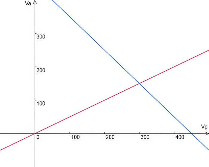
The two-trains plot turns two equations into two intersecting lines, making the solution visible as the point (300, 150). section 3.1.1
The geometry also reveals common system shapes:
- Intersecting hyperplanes can produce a single solution point. section 3.1.3
- Parallel hyperplanes indicate no exact solution when equations share dependent left sides but differ in their constants. section 3.1.3
- Coincident or underspecified hyperplanes can leave a line, plane, or other continuum of solutions rather than one point. section 3.1.3 section 3.10
A system can be written compactly as a coefficient matrix times a column vector, producing another column vector. Equation scaling, adding one equation to another, and swapping equations transform solvable systems toward an identity coefficient matrix, exposing the answer. Gaussian elimination and LU decomposition provide direct approaches; larger problems may instead use iterative solvers, whose convergence and stability matter. section 3.5.4 section 3.0 section 3.6
Choose the method to fit the workload. Small systems can be solved symbolically with SymPy and turned into formulas or code, avoiding library-call overhead in hot routines. Midsize systems suit elimination-based methods; sparse matrices can improve performance. Large systems may need iterative methods, convergence checks, and preconditioning. Symbolic formulas grow factorially and become impractical beyond very small dimensions. section 3.7.3 section 3.11
Ray–triangle intersection
A ray hits a triangle when a point on the ray equals a point on the triangle: P + td = A + ABu + ACv. Expanding this vector equation into x, y, and z produces three scalar equations for t, u, and v. Constraints t ≥ 0, u ≥ 0, v ≥ 0, and u + v ≤ 1 then reject intersections behind the ray or outside the triangle. Python and SymPy can solve the resulting small system. section 3.8.2 section 3.8.4
This pattern recurs throughout computational geometry: segment intersections, distances to triangles, edge offsets, custom projective transformations, smooth arc-and-line joins, and polynomial construction from derivative constraints can all be expressed through linear systems. section 3.8 section 4.7 section 5.3.2 section 11.6

