Local explanation accounts for one prediction rather than a model’s average behavior. It answers why a particular input received its result, helping people assess predictions, act on them, debug failures, and uncover possible data bias. This matters especially when a diagnostic or financial prediction affects a consequential decision. section 9.0 section 9.4
A local method is distinct from global explainability: global methods describe broadly relevant decision patterns across many examples, while local methods decompose or approximate the decision for a single example. Black-box ensembles often need a separate explanatory procedure; glass-box models can expose contributions directly through their structure. section 9.3 section 9.6
Common routes to a local explanation include:
- LIME, a model-agnostic local surrogate method. It generates examples near the input of interest, weights nearer examples more heavily, and fits an interpretable linear model to approximate black-box behavior in that neighborhood. Its explanation is the surrogate’s local feature contributions. section 9.4.1
- SHAP, a model-agnostic feature-attribution method. It assigns feature importance from each feature’s contribution to the prediction, using the cooperative-game-theory idea of Shapley values. section 9.4.2
- Explainable boosting machines (EBMs), which are trained as glass-box ensembles. Their additive single-feature and pairwise-feature components can be read directly as contributions for a specific classification or regression result, without approximating the model with LIME or SHAP. section 9.5.1 section 9.5
Explaining a subscription prediction
For Bank Marketing test example 3104, an EBM correctly predicts that a customer subscribes to a fixed-term deposit account with 66.1% confidence. A local explanation displays how individual features and selected feature interactions contribute positively or negatively to that result. LIME can similarly place positive feature contributions to the right of zero and negative contributions to the left for the same true-positive example. section 9.5.2 section 9.4.1
Figure 9.14 LIME creates a surrogate training set of examples in the locality of the example whose prediction needs to be explained. These examples are further weighted by their distance. This is indicated by the sizes of the surrogate examples, with closer examples getting higher weights (and shown larger). A weighted loss function is used to fit a linear surrogate model, which provides local explanations.
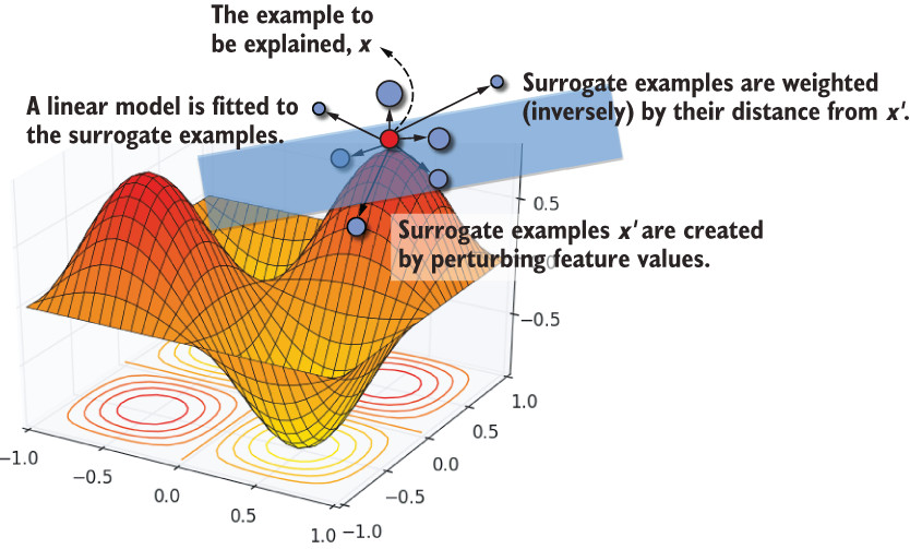
The diagram makes LIME’s locality concrete: sampled neighboring inputs receive distance-based weights before fitting the linear surrogate that explains one prediction. section 9.4.1
Figure 9.19 A waterfall plot to visualize Shapley values. The values along the left side of the plot show the feature values for test example 3104, while the text in the bars shows their Shapley values.
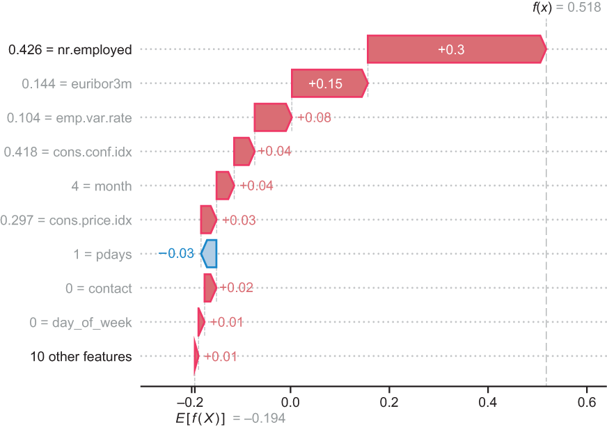
The waterfall visualization shows SHAP values for one test example, pairing its feature values with contributions that combine into the prediction. section 9.4.2
Local explanations are useful, but their meaning depends on the method. A LIME explanation describes a simple approximation around one point and explicitly balances fidelity against interpretability. SHAP attributes a prediction through feature contributions. An EBM instead makes its learned components available directly and can include important pairwise interactions, offering local and global views from the same model. section 9.4.1 section 9.5.1

