A log-link function models count or otherwise positive responses by connecting the logarithm of the expected response to a linear predictor. Instead of allowing the predictor to produce any real-valued result directly, it models log(y) = β₀ + β′x and inverts the relationship as y = e^(β₀ + β′x), keeping the response positive. section 7.1.2
The practical intuition is that features add on a logarithmic scale but multiply the response on its original scale. This suits a gentle exponential trend, such as event counts that grow with explanatory features, better than ordinary linear regression’s direct response scale. section 7.1.2
The link is selected together with assumptions about the target distribution:
- Poisson regression combines a linear model, the log link, and a Poisson distribution for count-valued labels. section 7.1.2 section 7.5
- Gamma regression uses the log link for positive, right-skewed continuous values. section 7.5
- Tweedie regression uses the log link for compound distributions arising in applications such as insurance, weather, and health analytics. section 7.5
From model to prediction
For count labels, fit a Poisson regression model to obtain β₀ and β, compute the linear predictor β₀ + β′x, and exponentiate it to obtain the predicted count mean. In scikit-learn, PoissonRegressor provides this workflow; one reported evaluation produced MSE 3.963 and mean absolute deviation 1.594, compared with 4.219 and 1.610 for ridge regression. section 7.1.2
Figure 7.4 Poisson regression (left) fits count-valued targets by assuming that the spread of the targets can be modeled by the discrete-valued Poisson distribution (right). More precisely, Poisson regression assumes that the predictions f(x) for an example x are distributed according to the Poisson distribution.
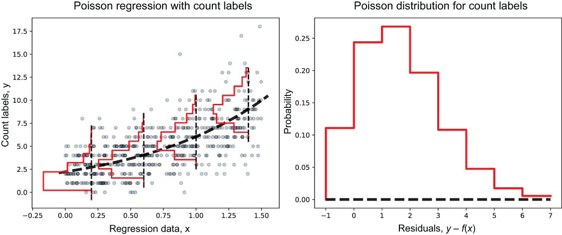
Compare the count-target trend and its Poisson-distribution spread with the continuous-target assumptions behind ordinary linear regression. section 7.1.2
