A link function lets a linear predictor handle targets that do not behave like ordinary continuous values. Rather than model a count or class label directly as β₀ + β′x, it transforms the target scale: g(y) = β₀ + β′x. Choosing g changes how linear feature effects become predictions on the original scale. section 7.1.2 section 7.1.4
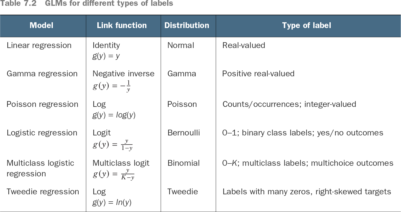
The choice follows the target’s distribution and the application. For count labels, the log link gives log(y) = β₀ + β′x, or y = e^(β₀ + β′x), matching an exponential mean trend with a Poisson distribution. For binary labels, the logit link transforms a probability into log-odds; inverting it produces the sigmoid used by logistic regression. section 7.1.2 section 7.1.3
Table 7.2 GLMs for different types of labels (view table figure)
Compare link–distribution pairs before selecting a generalized linear model: identity with normal targets, log with counts, and logit with binary labels are central examples. section 7.1.4
A generalized linear model combines four pieces:
- A probability distribution for the target, such as normal, Poisson, or Bernoulli. section 7.1.4
- A linear predictor η = β₀ + β′x, plus a link function g(y) = η. section 7.1.4
- A regularization function R(β) when coefficient control is needed. section 7.1.4
Reading logistic-regression effects
For diabetes classification, logistic regression models the log-odds of a positive diagnosis as a weighted sum of age and blood-glucose features. Increasing a feature shifts log-odds by its coefficient; exponentiating that shift expresses the corresponding change in odds. This preserves a linear, additive explanation while predicting class probabilities. section 9.1.3
Links also carry GLM intuition into nonlinear ensembles. For bike-sharing targets with many zeros and a right-skewed positive tail, a log link is suggested for a GLM; LightGBM and XGBoost can support link functions and distributions including Poisson, gamma, and Tweedie while learning beyond linear models. section 7.4.1