Binary classification needs predictions between 0 and 1 rather than unrestricted regression values. The logit link maps a class probability p to its log-odds, ln(p/(1-p)), allowing those values to be modeled as a linear combination of features. Applying the inverse link produces the sigmoid function, which converts the linear score back into a probability. section 7.1.3
Use the link to connect familiar regression machinery with classification:
- Model ln(p/(1-p)) = β0 + β′x, where the intercept and feature weights additively determine the log-odds. section 7.1.3 section 9.1.3
- Interpret p/(1-p) as the odds of the positive class and use the inverse-logit sigmoid to recover p. section 7.1.3
- Pair the model with the Bernoulli distribution, which represents yes/no outcomes rather than continuous values or event counts. section 7.1.3
Reading feature weights as odds changes
In a diabetes diagnosis model, increasing age by one raises log-odds by 0.5, multiplying the odds by e^0.5 ≈ 1.65. Increasing blood glucose by one lowers log-odds by 0.29, multiplying the odds by e^-0.29 ≈ 0.75. Positive weights increase positive-class odds; negative weights decrease them. section 9.1.3
Figure 7.5 Logistic regression (left) fits 0/1-valued targets by assuming that the spread of the targets can be modeled by the discrete-valued Bernoulli distribution (right). Observe how the prediction probabilities (the heights of the bars) of Class 0 and Class 1 change with the data.
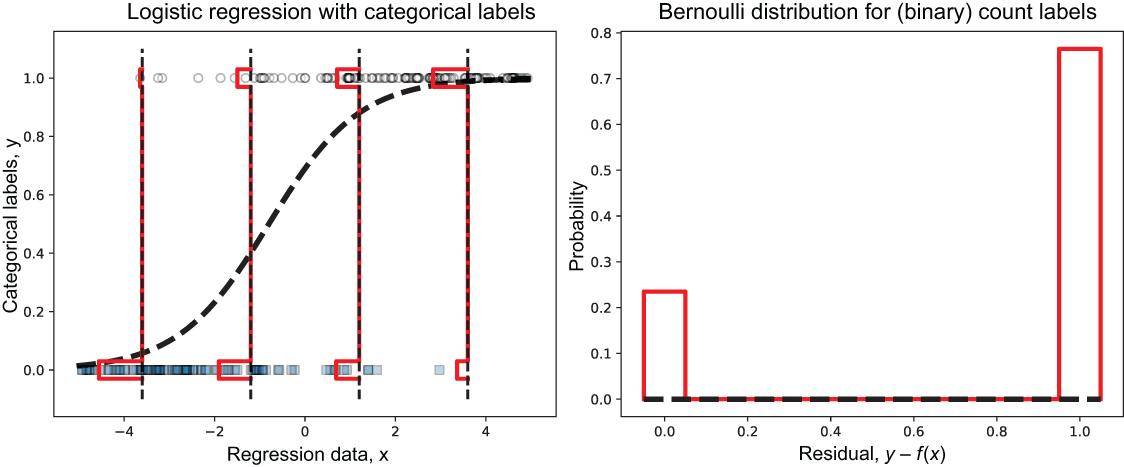
Visualizes logistic regression for 0/1 targets alongside Bernoulli probability distributions, showing how class probabilities change across the data. section 7.1.3
Listing 9.2 Training and interpreting logistic regression
from sklearn.datasets import load_breast_cancer
from sklearn.preprocessing import StandardScaler
from sklearn.linear_model import LogisticRegression
from sklearn.model_selection import train_test_split
import matplotlib.pyplot as plt
import numpy as np

bc = load_breast_cancer()                                              #1
X = StandardScaler().fit_transform(bc.data)                            #2
y = bc.target                                                          #2


Xtrn, Xtst, ytrn, ytst = train_test_split(X, y, test_size=0.15)
model = LogisticRegression(max_iter=1000, solver='saga', penalty='l1')
model.fit(Xtrn, ytrn)                                                  #3
ypred = model.predict(Xtst)
print('Accuracy = {0:5.3}%'.format(accuracy_score(ytst, ypred) * 100))

fig, ax = plt.subplots(figsize=(12, 4))

odds = np.exp(model.coef_[0]) - 1.                                     #4
ax.bar(height=odds,                                                    #5
       x=np.arange(0, Xtrn.shape[1])
for i, feature in enumerate(bc.feature_names):
    ax.text(i-0.25, 0, feature, rotation=90)
Provides a scikit-learn workflow that standardizes breast-cancer data, trains logistic regression, evaluates predictions, and supports coefficient-based interpretation. section 9.1.3
