Loss surface

As explained in Math and Architectures of Deep Learning

The geometric representation of a loss function over parameter space, where height indicates loss value for each parameter setting.

A loss surface is the geometric view of a loss function over parameter space, where each point’s height is the loss value for that parameter setting. section 9.2 section 9.1.1

Training treats this surface as the landscape to minimize: start from initial weights and biases, then move downhill toward lower loss with gradients. section 9.2 section 8.4.1

The representation connects to these ideas:

• level contours and level surfaces in geometric visualization. section 3.3.2
• gradients as the direction of maximum change and normals to contours. section 3.3.2
• optimization and momentum as methods for moving across the surface. section 9.2 section 9.2.4

Canyon analogy

The surface is compared to a canyon or ravine: optimization starts at a random point, then repeatedly steps downhill toward the lowest point. section 9.2 section 9.1.1

Figure 3.7 The domain of L(w₀, w₁) = √(w₀² + w₁²) shown as a heat map of function values. Gradients point radially outward, as shown by the arrowed line. The intensity of the heat map changes fastest along the gradient (that is, radii). This is the direction to follow to rapidly reach lower values of the function represented by the heat map.

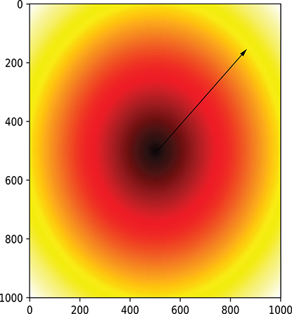
Shows a 2D loss field as a heat map, with gradients pointing radially and fastest change occurring along those directions. section 3.3.2

Figure 3.8 Gradient example in 3D: the function L(w₀, w₁, w₂) = L() = w₀² + w₁² + w₂². The levelsurfaces L() = constant are concentric spheres with the origin as their center. One such surface is partially shown in the diagram. ∇L() = k[w₀ w₁ w₂]^T—the gradient points radially outward. along the gradient, we go from one level surface to another, corresponding to maximum change in L(). Moving along any direction orthogonal to the gradient, we stay on the same level surface (sphere), which corresponds to zero change in the function value. D_θ() denotes the directional derivative along the displacement direction making angle θ with the gradient. If l̂ denotes this displacement direction, D_θ() = ∇L() ⋅ l̂.

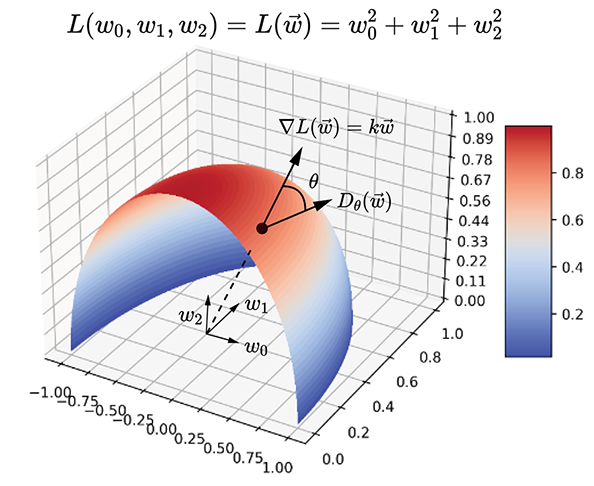
Extends the same idea to 3D, where level surfaces become concentric spheres and orthogonal movement leaves loss unchanged. section 3.3.2

Figure 3.9 Gradient example in 3D: the function L(w₀, w₁, w₂) = L() = w₀² + w₁². The level surfaces f() = constant are coaxial cylinders. One such surface is partially shown in the diagram: ∇L() = k[w₀ w₁ 0]^T. The gradient is normal to the curved surface of the cylinder along the outward radiusof the circle. Moving along the gradient, we go from one level surface to another, corresponding to themaximum change in L(). Moving along any direction orthogonal to the gradient, we stay on thesame level surface (cylinder), which corresponds to zero change in the function value.

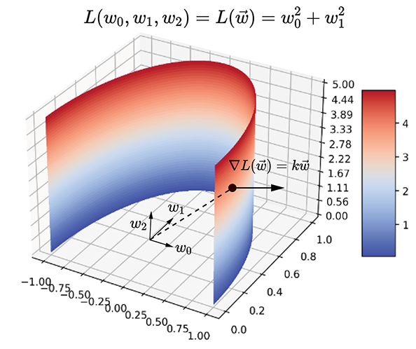
Shows a 3D case whose level surfaces are coaxial cylinders, emphasizing that gradients stay normal to the surface. section 3.3.2

How Math and Architectures of Deep Learning covers it

How deep it goes

Defines the surface, maps it to geometry, and links it to gradients and minimization, but stops short of algorithmic variants beyond basic descent.

Examples

Uses concentric circles, concentric spheres, coaxial cylinders, heat maps, and a canyon or ravine analogy.

What it assumes

Assumes vectors, weights, biases, gradients, and basic supervised-loss notation; introduces the geometric view from scratch.

What you can do after

Apply gradient descent and momentum to move toward lower loss on a neural network surface.

How it connects

Connects loss, gradients, level surfaces, optimization, and momentum.

liveBookmanning.com

Read Math and Architectures of Deep Learning on liveBook Get the book at manning.com

Also explained in

• 

  liveBookmanning.com
  Sutskever's ListA loss landscape is the function relating a model's parameter values to its loss across parameter space.

Compare how 2 books explain loss surface →

Related concepts

• gradient descentused by · Gradient descent is an iterative optimization method that updates parameters opposite the gradient of an objective function to reduce its value.
• momentumused by · Momentum is an optimization technique that incorporates a running history of gradients or parameter updates to smooth and accelerate movement during training.
• parameteruses · A model parameter is a numerical value, such as a weight or bias, that is learned or set to determine how a model computes outputs.
• hypersurfaceequivalent to · A surface of arbitrary dimension used here as the geometric shape of a loss surface in high-dimensional space.
• mean squared errorequivalent to · Mean squared error is the arithmetic mean of the squared differences between corresponding predicted and target numerical values.
• objective functionequivalent to · An objective function assigns values to candidate solutions, predictions, or parameter settings according to a criterion to be minimized or maximized.

This explainer was generated by Manning's knowledge graph from the text of Math and Architectures of Deep Learning. The section links point to the parts of the book it draws on.