Markov chain

As explained in Machine Learning Algorithms in Depth

A Markov model is a stochastic model in which the conditional distribution of future states depends on the present state rather than the full history.

A first-order Markov chain is a sequence of random states whose next-state distribution depends on the present state, not the full history: p(x₁,…,xT) = p(x₁)∏ₜ₌₂ᵀ p(xt|xt−1). The present state therefore contains the information needed to predict the next state. section 2.1.2 section 7.1

For K discrete states, define Aij = p(xt = j | xt−1 = i). The K × K transition matrix is stochastic: each row sums to 1. An initial distribution π₀ and A specify how state probabilities evolve: π₁ = π₀A, and repeated transitions give πt = π₀Aᵗ. When A does not change over time, the chain is time invariant. A stationary distribution π remains unchanged by a transition, so πA = π. section 2.1.2 section 7.1

Two states

Suppose the probability of leaving state 1 is α and the probability of leaving state 2 is β. Then A = [[1−α, α], [β, 1−β]]. Each row describes the possible next states from one current state and sums to 1. This small matrix makes both the one-step update and long-term distribution concrete. section 7.1

Figure 7.1 A two-state Markov model

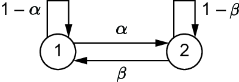
The two-state diagram shows which transition probability belongs to each directed change or stay in state. section 7.1

For page rank, states are web pages and transitions follow links in a graph. The link structure yields a sparse transition matrix; page rank is a stationary distribution computed at scale with power iteration. In Markov chain Monte Carlo, a chain is instead constructed so its stationary distribution is a target posterior. Hidden Markov models place a Markov chain over latent states and model observations emitted from them. section 2.1.2 section 7.8 section 1.4.1

How Machine Learning Algorithms in Depth covers it

How deep it goes

Defines first-order dependence and stochastic matrices, then develops state-distribution updates and long-term behavior; detailed sampling algorithms are deferred.

Examples

Uses a two-state transition diagram and a web-page link graph to illustrate transition probabilities.

What it assumes

Assumes conditional probability and matrix notation while defining first-order dependence and row-stochastic transitions.

What you can do after

Evaluate/understand it: form a discrete transition matrix, update state distributions, and interpret a stationary distribution in page rank or MCMC.

How it connects

Connects stationary distributions to page rank and Markov chain Monte Carlo, and latent-state chains to hidden Markov models.

liveBookmanning.com

Read Machine Learning Algorithms in Depth on liveBook Get the book at manning.com

Also explained in

• 

  liveBookmanning.com
  Statistics Every Programmer NeedsMarkov analysis is a technique for modeling transitions among a finite set of states using transition probabilities to predict future states.
• 

  liveBookmanning.com
  Fabulous Adventures in Data Structures and AlgorithmsA Markov process is a stochastic process in which the conditional distribution of the next state depends only on the current state.
• 

  liveBookmanning.com
  Optimization Algorithms: AI techniques for design, planning, and control problemsA stochastic model representing a sequence of states in which each transition probability depends only on the current state.

Compare how 4 books explain Markov chain →

Related concepts

• Markov decision processcontrasts with · A Markov decision process is a mathematical model of sequential decision-making defined by states, actions, probabilistic transitions, and rewards, with future dynamics depending on the current state and action.
• transition probabilityuses · A transition probability is the conditional probability that a stochastic process moves to a specified next state, possibly given its current state and an action.
• diffusion modelused by · A diffusion model is a generative model that learns to produce data by reversing a process that progressively adds noise to data.
• statehas part · State is information or a configuration describing the condition of a system, entity, or computation at a particular time and potentially influencing subsequent behavior or decisions.
• transition matrixuses · A transition matrix is a matrix whose entries represent the probabilities of moving between states in a stochastic process.

This explainer was generated by Manning's knowledge graph from the text of Machine Learning Algorithms in Depth. The section links point to the parts of the book it draws on.