Suppose you want to describe uncertainty about a preference, but cannot calculate its posterior distribution in a usable closed form. Markov chain Monte Carlo (MCMC) takes another route: it generates samples that approximate the posterior. Those samples can support estimates of its mean and credible intervals, as well as predictions and decisions. section 5.0
Imagine walking through a landscape of possible parameter values. A Markov chain makes each next step depend on the current position. MCMC designs that walk to spend time in regions according to their posterior density, concentrating effort where probability is high. Its samples are dependent, unlike ideal independent samples, but a well-explored chain can still approximate the target distribution. This avoids laying a grid across every possible value—a task that grows rapidly as dimensions are added. section 5.5 section 5.7
Figure 5.3 Differences between i.i.d. sampling (left) and MCMC (right). MCMC generates a chain of dependent samples (order indicated by arrows) that approximates the distribution.
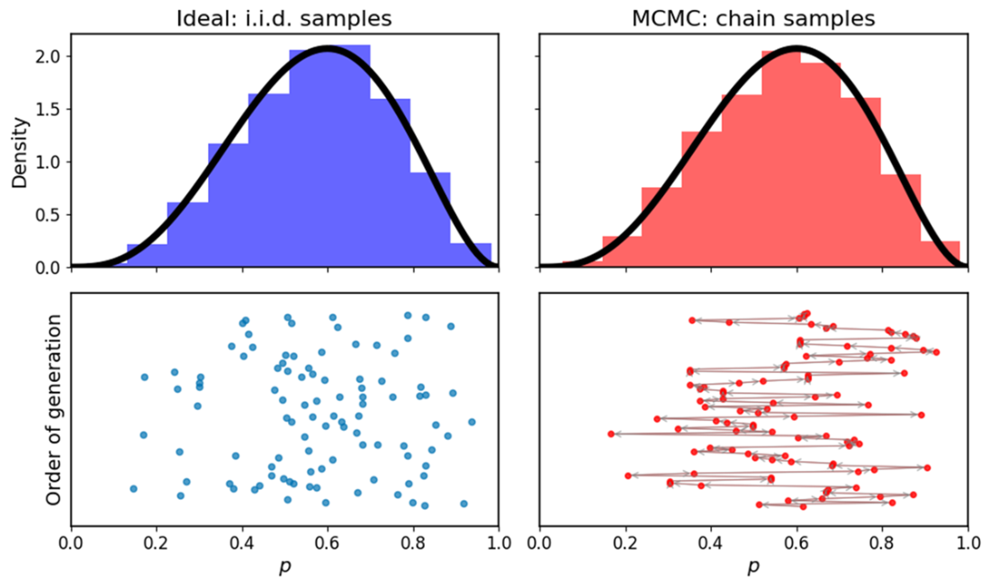
Compare independently scattered samples with the ordered MCMC walk; both panels approximate the same distribution. section 5.5
Metropolis–Hastings makes the walk concrete. Start at a possible value, propose a nearby one, and compare their posterior densities. For a Normal proposal centered on the current value, accept the move with probability min(1, proposed density ÷ current density); otherwise, record the current value again. Repeat. The ratio still works when the posterior density is known only up to a shared constant. The proposal and accept/reject rule together determine how the chain explores. section 5.6 section 5.7
Sampling an uncertain preference
For a tea-versus-coffee preference, begin with a uniform Beta(1, 1) prior and observe 3 preferences out of 5. A small NumPy implementation can propose values of the preference probability and retain or reject each move. PyMC expresses the prior and Binomial observation directly, then draws posterior samples with pm.sample(). section 5.6 section 5.8
samples = np.empty(n_samples)                #A
samples[0] = initial                         #A
current_post = unnormalized_posterior(       #B
    initial
)

for t in range(1, n_samples):
    proposal = np.random.normal(             #C
        samples[t-1], proposal_stddev
    )
    proposal_post = unnormalized_posterior(  #D
        proposal
    )

    r = proposal_post / current_post         #E
    if np.random.rand() < r:                 #F
        samples[t] = proposal
        current_post = proposal_post
    else:                                    #G
        samples[t] = samples[t-1]
Follow the NumPy loop from a Normal proposal through the density ratio to an accepted move or a repeated value. section 5.6
Do not treat every generated value as trustworthy. Discard early burn-in samples while the chain moves away from its starting point, and run multiple chains from different positions. Check whether chains converge to the same stationary distribution: R̂ near 1 is reassuring, while a value above 1.05 is a warning not to use the samples. Check effective sample size (ESS) and trace plots for inefficient exploration, then use posterior predictive checks to compare simulated and observed data. PyMC handles sampling and burn-in; ArviZ provides summary diagnostics. section 5.9 section 5.10 section 5.11 section 5.14
MCMC is useful beyond a simple preference model: posterior samples of Bayesian neural-network parameters can produce predictions with credible intervals that widen where observations are scarce. The trade-off is time. Chains may need many steps for complex models or large datasets; variational inference is often faster but uses a potentially less faithful approximation. section 10.3 section 6.14



