Nine-point transformation

As explained in Geometry for Programmers

A nine-point transformation is a two-dimensional polynomial transformation whose two coordinate polynomials each contain nine coefficient terms.

A nine-point transformation maps (xi, yi) to (xt, yt) using two biquadratic polynomials. Each polynomial contains 3 × 3 = 9 terms, covering degrees 0, 1, and 2 in both variables. section 8.1.1

Its practical structure is:

• Represent xt and yt with separate coefficient sets, a11–a19 and a21–a29. section 8.1.1
• Fit the transformation from corresponding points through 18 equations, two for each polynomial member. section 8.1.1
• Solve the x and y coefficient systems independently because their coefficients do not mix. section 8.1.1

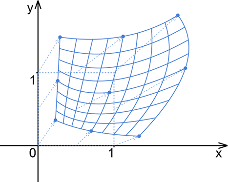
Figure 8.2 An example of a biquadratic transformation of the standard square

A figure illustrates how a biquadratic transformation can reshape a standard square. section 8.1.1

How Geometry for Programmers covers it

How deep it goes

Defines the nine terms and derives the eighteen-equation setup, then stops short of a complete symbolic solution.

Examples

Uses a standard-square figure and SymPy-style coefficient equations to illustrate the transformation.

What you can do after

Evaluate paired biquadratic coordinate formulas and organize their fitting equations into independent x and y systems.

How it connects

Connects polynomial transformation with bilinear transformation, biquadratic polynomial, and symbolic solving.

liveBookmanning.com

Read Geometry for Programmers on liveBook Get the book at manning.com

Related concepts

• biquadratic transformationkind of · A biquadratic transformation is a mapping described by expressions that are quadratic in each of two input variables.

This explainer was generated by Manning's knowledge graph from the text of Geometry for Programmers. The section links point to the parts of the book it draws on.