Biquadratic transformation

As explained in Geometry for Programmers

A biquadratic transformation is a mapping described by expressions that are quadratic in each of two input variables.

A biquadratic transformation maps two input variables using terms quadratic in each variable, including x²y², x²y, xy², and constant terms. Applying it to a standard square produces a flexible nonlinear shape, but determining its coefficients requires solving a nine-equation system for each output coordinate. section 8.1.1

The straightforward construction has practical limits:

• Solves two independent nine-equation systems instead of one system of eighteen equations. section 8.1.1
• Becomes harder to scale as polynomial degree rises: bicubic systems require sixteen equations, while biquartic systems require twenty-five. section 8.1.1
• Accumulates floating-point error as symbolic or numerical systems grow, motivating expression optimization with Herbie. section 8.1.1

Coefficient system

A typical output coordinate uses nine coefficients: a11x²y² + a12x²y + a13x² + a14xy² + a15xy + a16x + a17y² + a18y + a19. Substituting nine corresponding input and target points yields the equations solved symbolically. section 8.1.1

Figure 8.2 An example of a biquadratic transformation of the standard square

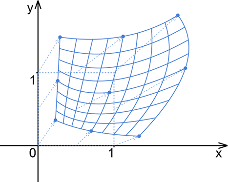
Use the figure to inspect how a biquadratic transformation reshapes the standard square. section 8.1.1

How Geometry for Programmers covers it

How deep it goes

Works through coefficient systems and scaling limits, but defers simpler alternative formulas and detailed numeric optimization.

Examples

Uses a standard-square figure and a nine-coefficient symbolic system built from corresponding input and target points.

What you can do after

Evaluate coefficient-system size, geometric flexibility, and numerical trade-offs when choosing polynomial transformations.

How it connects

Connects biquadratic transformations with bilinear, bicubic, biquartic, polynomial transformations, SymPy, and floating-point error.

liveBookmanning.com

Read Geometry for Programmers on liveBook Get the book at manning.com

Related concepts

• inverseused by · An inverse is a value or operation that reverses the effect of another value or operation under a specified composition rule.
• signed distanceuses · A signed distance is a distance from a geometric boundary or separator assigned a positive or negative sign according to which side contains the point.
• nine-point transformationincludes · A nine-point transformation is a two-dimensional polynomial transformation whose two coordinate polynomials each contain nine coefficient terms.
• biquadratic polynomialimplemented by · A biquadratic polynomial is a two-variable polynomial with degree at most two in each variable.

This explainer was generated by Manning's knowledge graph from the text of Geometry for Programmers. The section links point to the parts of the book it draws on.