Observational joint distribution

As explained in Causal AI

An observational distribution is the probability distribution of variables generated under ordinary observation without externally intervening on the system.

An observational joint distribution is the true probability distribution of variables as they arise through ordinary observation, without externally intervening on the system. It describes how complete combinations of observed values occur, such as whether Jenny throws a rock, Brian throws a rock, and a window breaks. section 2.3.2

Observed data provide an empirical joint distribution: the proportions of combinations in a finite sample. Sampling repeatedly from the observational distribution makes those proportions converge toward the underlying probabilities, but a small sample can contain no instance of an outcome that still has nonzero probability. section 2.3.2

Use the distribution to keep three probability objects distinct:

• Empirical joint distribution: finite-sample counts or proportions calculated from observed rows. section 2.3.2
• Observational joint distribution: the underlying distribution that generates those observed rows. section 2.3.2
• Full joint distribution: the joint distribution over observed and latent variables; marginalizing latent variables recovers the observational distribution. section 2.3.2

In causal analysis, observational data are samples from a level-one distribution, while an intervention query belongs to a higher level of the causal hierarchy. Identification therefore seeks a level-one estimand that can be computed from the observational distribution under an explicit causal model and its assumptions. section 11.3

Conditioning versus intervening

A language model can generate an observational sample conditioned on a Prince vignette, P(Kingdom|Prince=x), where observing the Prince constrains likely Kings. Applying a do-intervention fixes the Prince while removing the incoming causal edge, allowing greater variation in generated Kings and Kingdoms. section 13.3.3

Table 2.4 Assume this is the true observational joint distribution.

	jenny_throws_rock	brian_throws_rock	window_breaks	probability
1	False	False	False	0.25
2	True	False	False	0.15
3	False	True	False	0.15
4	True	True	False	0.05
5	False	False	True	0.00
6	True	False	True	0.10
7	False	True	True	0.10
8	True	True	True	0.20

Inspect a concrete eight-outcome probability table for the assumed observational joint distribution. section 2.3.2

Figure 2.24 Sampling from the observational joint distribution produces the observed data and empirical distribution.

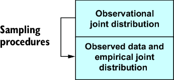
Trace how sampling from the observational distribution produces observed data and its empirical distribution. section 2.3.2

How Causal AI covers it

How deep it goes

Defines the distribution, contrasts it with empirical and full joint distributions, and stops short of treating it as an intervention distribution.

Examples

Uses rock-throwing data, an online-game dataset, and language-model generations to contrast observed, conditioned, and intervened distributions.

What you can do after

Evaluate observed data as samples from a joint distribution and apply them in DoWhy-based causal identification workflows.

How it connects

Connects empirical distribution, latent variables, full joint distribution, causal model, estimand, and interventional distribution.

liveBookmanning.com

Read Causal AI on liveBook Get the book at manning.com

Related concepts

• joint probability distributionproduced by · A joint probability distribution specifies probabilities or densities for combinations of values taken simultaneously by multiple random variables.
• functional constraintused by · A functional constraint is a testable restriction on an observed probability distribution implied by a causal graph, including one obtained after accounting for latent variables.
• intervention distributioncontrasts with · An intervention distribution is the probability distribution of variables generated by externally setting or changing one or more variables in a causal model.
• probability distributionkind of · A probability distribution is a mathematical specification assigning probabilities to the possible values or outcomes of a random variable, with total probability one.

This explainer was generated by Manning's knowledge graph from the text of Causal AI. The section links point to the parts of the book it draws on.