Suppose one dataset contains a sparse cluster and two dense clusters close together. With DBSCAN, a small neighborhood radius fragments the sparse cluster; a larger one merges the dense pair. OPTICS addresses this problem by ordering points and recording reachability distances, so clustering structure can be examined across radii rather than fixed by one radius at the outset. section 12.4
Figure 12.14 An example of a dataset with areas of heterogeneous density for which it’s not possible to find a single value of ϵ that fits all areas. The dataset has a low-density cluster in the left area and two high-density clusters, close to each other, in the top-right corner. (Left) With a low value of ϵ, the low-density cluster is broken into many small clusters surrounded by noise. (Right) With higher values, the two clusters on the right are merged. There is no value for which these clusters are correctly separated and at the same time the one on the left is recognized as a single cluster.
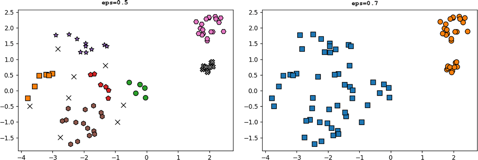
Compare the two radius choices: neither preserves the sparse cluster while separating the dense pair. section 12.4
OPTICS takes a minimum point count and εMAX. Unlike DBSCAN’s radius, εMAX is the largest neighborhood radius considered while building the ordering; a separate cutoff ε can later select a flat clustering, up to εMAX. A point’s core distance expresses how far its neighborhood must extend to contain enough points. For a neighbor q of a core point p, its candidate reachability distance is max(coreDistance(p), distance(p, q)). A point without enough neighbors inside εMAX is not a core point and cannot expand the frontier. section 12.4.2
To construct the ordering:
- Initialize every reachability distance as undefined, an empty ordering, and a spatial index for radius queries. section 12.4.2
- Choose an unprocessed point and append it to the ordering. If it is a core point, examine its unprocessed neighbors and place them in a priority queue keyed by their best known reachability distances. section 12.4.2
- Repeatedly process the queued point with the smallest reachability distance. When processing a core point reveals a shorter route to an unprocessed neighbor, lower that neighbor’s queue priority. Start again from an unprocessed point when the frontier is empty. section 12.4 section 12.4.2
Figure 12.17 A reachability plot. The top chart shows the clustered dataset, the bottom half the reachability distances of points in the dataset, in the same order as points are processed by OPTICS. Outliers are shown in black (with an X marker in the top plot); clusters are assigned the same shade (or color, if you are reading the digital version) in both charts (dashed lines link clusters across the charts). The reachability distances are computed by OPTICS given parameters minPoints and ϵMAX. Further, there is a parameter ϵ that determines the cutoff point for reachability distances and therefore the actual partitioning into clusters.
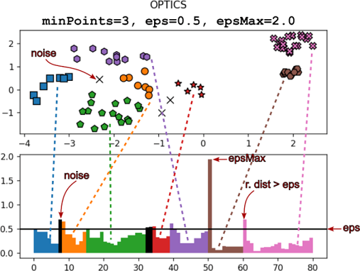
Read the reachability distances in processing order, then compare them with a cutoff ε to see how a flat partition is selected. section 12.4.2
Changing ε changes the flat clustering without rerunning the ordering. Increasing it generally merges clusters, but one global cutoff can still merge an unwanted pair before another pair joins. The hierarchical view records these merges; a dendrogram can then be cut at different thresholds in different branches. Choosing sensible branches may require domain knowledge rather than a single automatic radius choice. section 12.4.4
The trade-off is cost. Each point is processed once, but neighborhood queries and frontier priorities need updates. A large εMAX considers more neighbors and leaves more clustering options open, while making queries and the queue more expensive. Worst-case running time is quadratic; with an appropriate εMAX, average running time can be as low as O(n log n). Retaining and exploring the hierarchy adds memory and computation beyond the core algorithm. section 12.4.2 section 12.4.5
