A policy gradient method directly adjusts a parameterized policy to increase expected return. It is useful when decisions are continuous or high-dimensional: a cooling controller, for example, must choose fan speeds and valve openings across interconnected zones, rather than select from a small menu of actions. section 9.0 section 9.8
A stochastic policy produces a probability distribution over actions for a given state. For continuous control, it can output the mean and standard deviation of a Gaussian distribution, then sample an action. This gives the policy a way to explore without enumerating every possible action. section 9.1 section 9.8
The policy gradient estimates how to change the policy parameters using sampled trajectories. For each action, the gradient of its log-probability points toward making that action more likely; a return weights that direction. Good outcomes reinforce the decisions that produced them, while poor outcomes can suppress them. The estimate does not require knowing the environment’s transition dynamics. section 9.2 section 9.8
REINFORCE is a practical policy gradient algorithm:
- Sample actions from the policy and collect complete trajectories of states, actions, and rewards. section 9.8
- Calculate discounted returns and use them to weight the actions’ log-probability gradients. section 9.3
- Update the policy parameters in the direction of the estimated gradient, then repeat with new trajectories. section 9.8
Figure 9.4 The REINFORCE algorithm core steps.
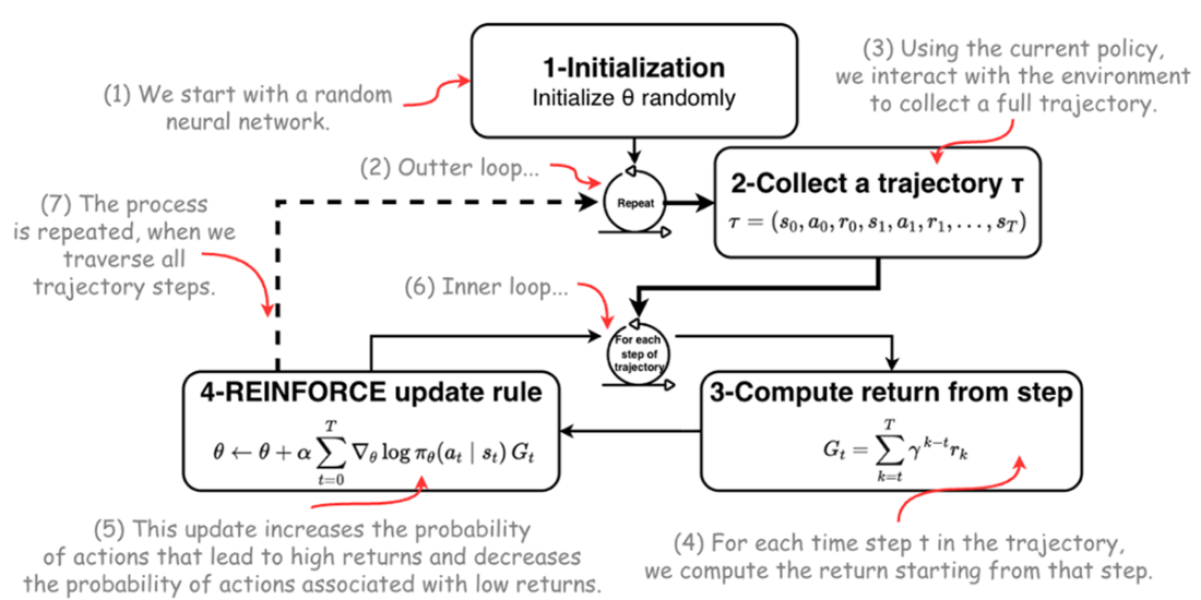
The diagram brings the sampling, return calculation, and policy update together. section 9.3
Plain REINFORCE can have high-variance updates: a trajectory’s return may reflect many events, not just one action. A baseline reduces variance by comparing the return with an expectation. In an actor-critic design, a value network supplies that baseline, and the actor uses the resulting advantage to update the policy. Entropy regularization can also be included in the training objective. section 9.8 section 9.7
Cooling an eight-zone data center
The controller observes eight features per zone, including temperature, workload, neighboring temperature, and previous controls. It chooses a fan speed and valve opening for each zone: 16 continuous actions in total. The reward penalizes energy use and temperature or pressure violations over a simulated 24-hour horizon. A Transformer actor-critic combines a Gaussian policy with a value baseline to learn from these interactions. section 9.7
Listing 9.10 Policy gradient update with value baseline and entropy regularization
data = buffer.get_tensors()
T, B = returns.shape
obs_flat = data['observations'].view(
    T * B, config.n_zones, -1)                        #A
actions_flat = data['actions'].view(
    T * B, config.n_zones, 2)  #A
returns_flat = returns.view(T * B)
advantages_flat = advantages.view(T * B)

returns_mean = returns_flat.mean()
returns_std = returns_flat.std() + 1e-8
returns_normalized = (
    returns_flat - returns_mean) / returns_std  #B

log_probs, entropy, values = \
    model.evaluate_actions(obs_flat, actions_flat)  #C

policy_loss = -(
    log_probs * advantages_flat.detach()).mean()  #D

value_loss = F.mse_loss(
    values, returns_normalized.detach())  #E

entropy_loss = -entropy.mean()  #F

total_loss = (policy_loss +
    config.value_coef * value_loss +
    config.entropy_coef * entropy_loss)  #G

optimizer.zero_grad()
total_loss.backward()  #H
torch.nn.utils.clip_grad_norm_(
    model.parameters(), config.max_grad_norm) #I
optimizer.step()
The update combines an advantage-weighted policy loss with value and entropy terms. section 9.7
Direct policy optimization avoids discretizing continuous controls and can represent useful randomized strategies, such as unpredictable patrol routes. The trade-off is that policy gradients can have noisy estimates, converge to local optima, and use more samples than DQN. section 9.1 section 9.0