Polynomial degree is the highest power of its variable with a nonzero coefficient. In canonical form, a polynomial lists powers from highest to lowest: x³ − 2x² + 4 has degree 3, so it is cubic. Zero coefficients may be written explicitly, but they do not change the degree. Degree is a quick way to describe both the expression’s shape and the number of coefficients that must be determined. section 6.1
Degree gives useful geometric expectations. A degree-n polynomial has at most n roots, where its graph meets the x-axis. Its derivative has degree one lower, so each added degree can introduce at most one additional extremum, or bump. Odd-degree polynomials must have at least one root; even-degree polynomials may have none. section 6.1.2 section 6.1.3
Degree, roots, and turns
A linear polynomial can have one root and no extrema. A quadratic can have up to two roots and one extremum. A cubic can have up to three roots and two extrema because its derivative is quadratic. This does not promise that every possible root or bump appears; it sets an upper bound that helps when reading a plotted curve. section 6.1.1 section 6.1.2
For interpolation, degree controls how many independent coefficients are available. A polynomial of degree N−1 has N coefficients, so N points generally determine one unambiguous interpolating polynomial. Raising the degree provides extra freedom for restrictions beyond passing through points, but it also loses that unambiguity. A Vandermonde matrix turns the point constraints into a linear system for those coefficients. section 6.3.1 section 7.1
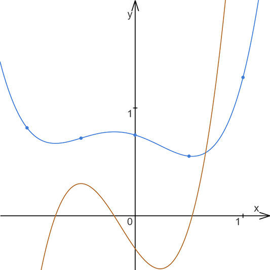
Compare the degree of an interpolating polynomial with the maximum number of extrema it can develop between data points. section 6.3.2
Higher degree is not automatically better. Interpolating N points with degree N−1 can create up to N−2 bumps, and the resulting curve may oscillate strongly near the interval ends as more points are added. For large data sets, this Runge’s phenomenon can make one global polynomial a poor practical choice; splines or rational interpolants are alternatives. Degree also selects the target model in least-squares approximation, such as degree 1 for a linear trend. section 6.3.2 section 6.2.3
Degree remains a design choice in piecewise curves as well. In NURBS and polynomial splines, increasing the common degree increases continuity while reducing the number of curve segments obtainable from a fixed set of control points. First-degree curves are piecewise linear; second-degree curves preserve C1 continuity, while higher degrees raise continuity further. section 7.3.1