A polynomial function builds an output from constant coefficients, a variable, addition, multiplication, and non-negative powers. In canonical form, terms are ordered by descending power: P(x) = aₙxⁿ + … + a₁x + a₀. Zero, one, and negative coefficients are all allowed; the highest nonzero power is the degree. section 6.1
Polynomials are useful digital clay for geometry: they are simple enough to compute cheaply, yet flexible enough to describe curves, approximate other functions, and interpolate points. Their coefficients are also a compact representation, so one formula can be stored as a short coefficient list. section 1.2 section 6.0 section 6.1.3
The same polynomial can be viewed and evaluated in several practical ways:
- Canonical form exposes coefficients and degree, such as C(x) = x³ − 2x² + 4. section 6.1
- Factored form exposes roots: in (x − r₁)(x − r₂)(x − r₃), each r makes the polynomial equal zero. section 6.1
- Horner’s scheme nests multiplications, P(x) = ((ax + b)x + c)x + d, reducing a cubic evaluation from six multiplications to three. section 6.1
A root is an x value where P(x) = 0, geometrically where the graph meets the x-axis. A degree-n polynomial has at most n roots. Linear polynomials have one root when their slope is nonzero; quadratics may have zero, one, or two; odd-degree polynomials have at least one. section 6.1.1 section 6.1.3
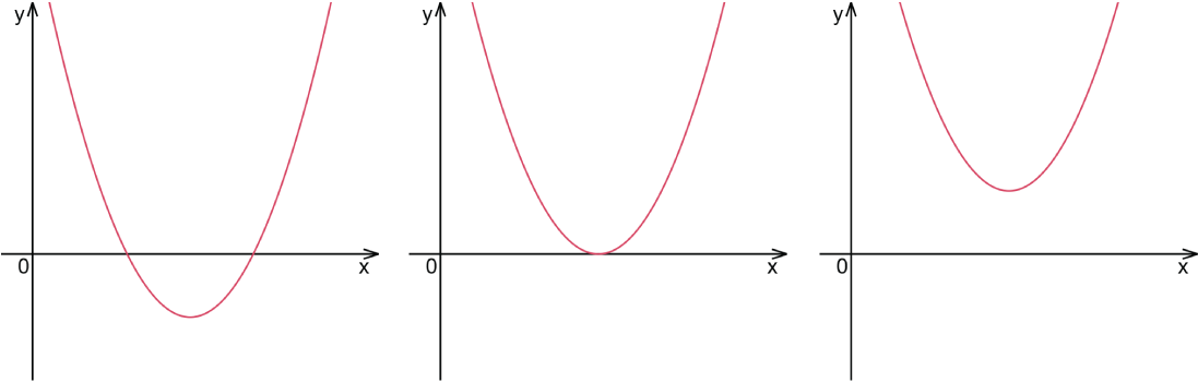
Compare the possible x-axis intersections of a quadratic polynomial: crossing twice, touching once, or missing the axis. section 6.1.1
Differentiation preserves the polynomial form while lowering degree by one, except that a linear polynomial becomes a constant. Roots of the derivative help locate possible extrema: when the derivative changes from negative to positive or positive to negative, the original graph has a local minimum or maximum. A derivative root alone is not enough; it may only touch the axis. section 6.1.2
For computation, polynomial functions replace more expensive functions with additions and multiplications. Raising or lowering degree creates a practical precision-versus-performance trade-off. In interpolation, a polynomial passes exactly through supplied points; normally N points determine an unambiguous polynomial of degree N − 1. section 6.2 section 6.7
Curve with point and tangent constraints
A cubic can be fitted through two points while also matching specified tangent slopes there. Point conditions constrain P(xᵢ); tangent conditions constrain P′(xᵢ). These become linear equations in the unknown coefficients, allowing a curve to be shaped rather than merely forced through points. section 7.1.1
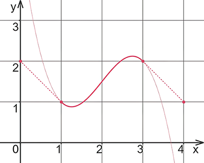
The figure shows a cubic whose coefficients are determined by two endpoint positions and two tangent directions. section 7.1.1