Pooling

As explained in Inside Deep Learning: Math, Algorithms, Models

A neural-network operation that downsamples local neighborhoods by aggregating their values.

Pooling downsamples local neighborhoods by aggregating their values. In a CNN, it reduces the spatial detail passed to later layers and makes predictions more robust when image content shifts slightly. This matters because a later fully connected layer tends to associate features with specific locations, while pooling preserves useful spatial evidence across nearby positions. section 3.5 section 3.8

Max pooling applies a sliding window over each channel:

• For a K × K region, select its largest value and write it to the output. With a matching stride, each spatial dimension shrinks by roughly K. section 3.5
• Use the stride to control how far the window moves; pooling and convolution both expose this setting. section 3.8
• Treat ordinary max pooling as a tradeoff: it improves shift robustness and enlarges later receptive fields, but can discard more information than necessary. section 14.1
• For severe aliasing, pool with stride=1 and padding, then blur and downsample with a stride-2 convolution; a binomial filter weights nearby values more heavily. section 14.1.2

A shift-sensitive classifier

Shift an MNIST digit one pixel with `np.roll`, then evaluate it through a PyTorch model. The probability assigned to the correct class can fall from 0.7816 for the original image to 0.4428 or 0.3153 after small shifts; pooling addresses this location sensitivity. section 3.5

PyTorch anti-aliased pooling pattern

Apply `F.max_pool2d(x, kernel_size, stride=1, padding=kernel_size//2)`, then pass the result through `BlurLayer(kernel_size=int(1.5*shrink_factor), stride=shrink_factor)`. This keeps the local maxima behavior while mixing neighboring information before reduction. section 14.1.2

Figure 14.2 An approach to max pooling that helps mitigate aliasing: also called anti-aliasing. First we do max pooling with a stride of 1 to get an output the same size as the input. Then we apply a blurring kernel/convolution with a stride of 2, which shrinks the output to the desired size and maintains the behavior of max pooling but allows us to delineate that the three outputs came from three different inputs. This approach captures more information than naive max pooling.

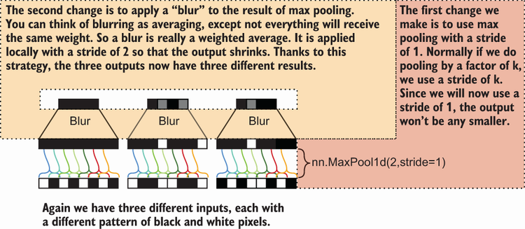
Visualizes the anti-aliasing sequence: stride-1 max pooling preserves a full-size intermediate representation, then blurring with stride 2 reduces it while distinguishing inputs that naive pooling makes identical. section 14.1.2

How Inside Deep Learning: Math, Algorithms, Models covers it

How deep it goes

Explains max pooling, stride, receptive fields, aliasing, and an anti-aliased replacement with PyTorch implementation patterns.

Examples

Uses shifted MNIST digits, K-sized max-pooling diagrams, and a zebra image to expose spatial sensitivity and aliasing.

What it assumes

Assumes CNNs, image tensors, convolution, and basic PyTorch while grounding pooling in spatial data and model architecture.

What you can do after

Apply pooling via PyTorch and diagnose information loss by comparing naive max pooling with blur-based downsampling.

How it connects

Connects pooling with convolution, translation invariance, receptive fields, aliasing, blurring, and transposed convolution.

liveBookmanning.com

Read Inside Deep Learning: Math, Algorithms, Models on liveBook Get the book at manning.com

Also explained in

• 

  liveBookmanning.com
  Natural Language Processing in Action, Second EditionA pooling layer is a neural-network layer that aggregates neighboring activations to reduce their representation while retaining salient information.
• 

  liveBookmanning.com
  Math and Architectures of Deep LearningA downsampling operation on feature maps that reduces spatial resolution, often by local averaging or max selection.
• 

  liveBookmanning.com
  Build a Text-to-Image Generator (from Scratch)A pooling layer aggregates values within local spatial windows to produce a reduced or transformed feature representation.
• 

  liveBookmanning.com
  Evolutionary Deep Learning: Genetic algorithms and neural networksPooling is a neural-network operation that aggregates values within local regions to reduce spatial or feature-map dimensions.
• 

  liveBookmanning.com
  Graph Neural Networks in ActionA graph operation that reduces a collection of representations to a smaller representation, often for graph-level prediction.
• 

  liveBookmanning.com
  Deep Learning with PyTorch, Second EditionA downsampling technique that reduces spatial resolution by aggregating local regions of a feature map.
• 

  liveBookmanning.com
  AI-Powered SearchPooling is the aggregation of multiple representation values into a single lower-level or fixed-size representation.

Compare how 8 books explain pooling →

Related concepts

• convolutional neural networkused by · A convolutional neural network is a neural-network architecture that applies learned convolutional operations to extract patterns from structured data.
• max poolingincludes · Max pooling is an aggregation operation that replaces each local or grouped region with its maximum value, often to downsample a representation.
• downsamplingequivalent to · Downsampling is the reduction of data quantity, spatial resolution, temporal resolution, or sampling rate by retaining, selecting, or aggregating fewer representative values or observations.
• upsamplingalternative to · Upsampling is a process that increases the number, density, or spatial or temporal resolution of samples or values in a dataset or representation by adding, duplicating, or estimating them.
• gradientuses · A gradient is the vector of partial derivatives of a scalar function with respect to its variables, indicating its local rate and direction of change.

This explainer was generated by Manning's knowledge graph from the text of Inside Deep Learning: Math, Algorithms, Models. The section links point to the parts of the book it draws on.