Positivity assumption

As explained in Causal Inference for Data Science

The positivity assumption is the condition that every treatment has a nonzero and non-unit probability of being assigned at every confounder value that occurs in the population.

Before comparing treatments, ask a practical question: within every relevant kind of person or situation, have both alternatives actually occurred? The positivity assumption says that for every confounder profile present in the population, each treatment has a probability strictly between 0 and 1 of being assigned. Without such variation, a causal effect requires guessing about an unobserved situation rather than learning from comparable cases. section 2.2.6 section 5.0

A treatment never tried for small stones

Suppose treatment A was used only for large kidney stones. Even if outcomes are available for large stones, there is no evidence for how A works on small stones: P(T=A|Size=small)=0. More observations may fill a sparse cell caused by chance, but they cannot fix a treatment policy that deliberately never assigns A to small-stone patients. section 2.2.6

Positivity is needed when using adjustment to turn observational comparisons into causal estimates. It is distinct from a causal graph: a DAG can identify confounders and adjustment variables, but arrows do not reveal whether the data contain both treatments for every confounder pattern. Check treatment variation after defining the causal question and graph. section 2.6 section 3.2.5

A useful operational check is:

• List the confounders that define the situations to be compared, using domain knowledge rather than prediction convenience. section 3.2
• Look for subgroups represented in only one treatment group; those cases have no counterpart under the alternative. section 5.1.2
• Restrict the analysis to common-support cases when overlap exists only for a subset; do not claim an effect outside that subset. section 3.2.5 section 3.6
• Recognize that many confounders make positivity harder: every observed combination needs treatment variation, while combinations grow rapidly. section 2.5.5

Discounts across purchase-frequency groups

If frequent purchasers always receive large discounts and infrequent purchasers always receive small ones, discount size is inseparable from purchase history. Randomly assigning both discount sizes within both frequency groups preserves the comparisons needed to estimate the discount effect. section 3.3.2

With continuous or numerous confounders, exact matches are often unrealistic. Similar cases may be treated as comparable, but that judgment is supported rather than proven by data. Binning a continuous variable can help inspect overlap, although wide bins combine meaningfully different cases and narrow bins leave too few observations. section 5.1.3 section 5.2.3

Figure 5.9 The distribution of propensity scores between the two groups shows no overlap, indicating that there are no matches between the groups. Consequently, we cannot calculate ATEs.

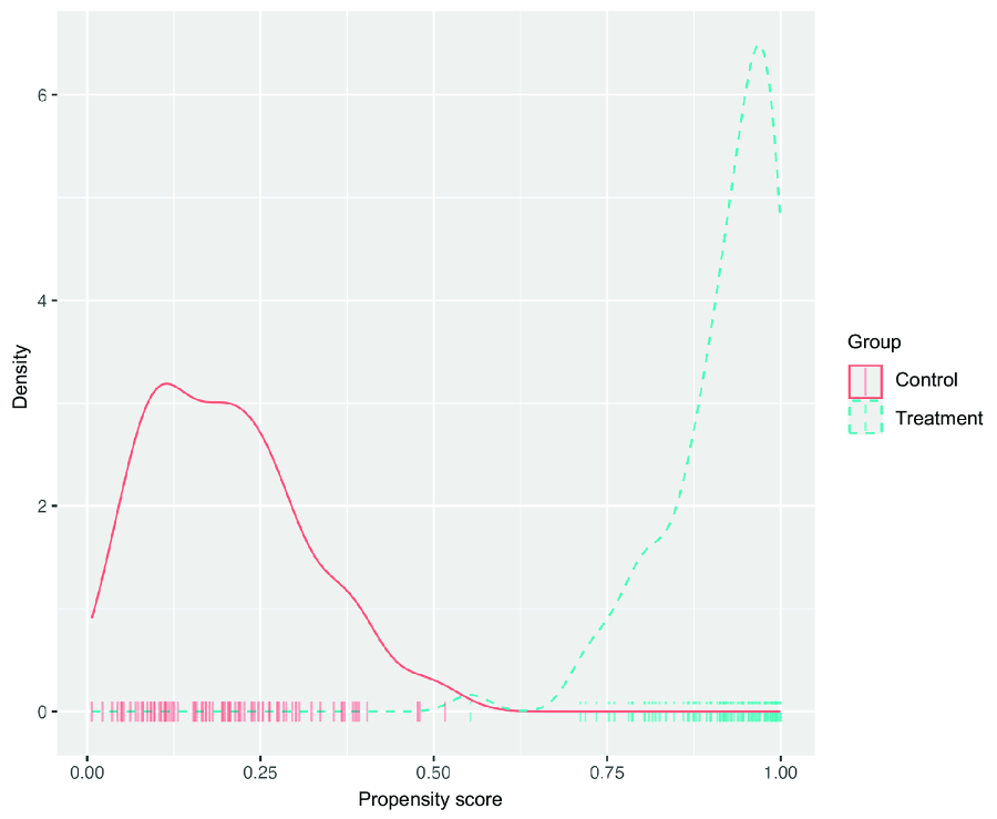
Compare the treatment and control propensity-score distributions: no overlap means no comparable cases and no ATE for that population. section 5.3.3

A propensity score summarizes the probability of treatment from a confounder profile. Scores near 0 or 1 signal that treatment is essentially determined for that profile; overlap between treatment groups supports comparison. Propensity scores can replace an unwieldy check across every raw confounder combination, then be reused for average treatment-effect calculations. section 5.1.2 section 5.3.3 section 5.7

How Causal Inference for Data Science covers it

How deep it goes

Defines the probability condition, explains design failures and common support, and operationalizes assessment with propensity scores.

Examples

Uses kidney-stone treatments, advertising platforms by topic, patient age and blood pressure, and customer discounts.

What it assumes

Assumes a causal question and identified confounders, while teaching positivity from treatment assignment patterns and comparable cases.

What you can do after

Evaluate/understand whether a causal comparison is supportable, restrict it to common support, or stop when groups lack overlap.

How it connects

Connects adjustment formula, confounders, DAGs, matching, propensity scores, ATE, ATT, and randomized controlled trials.

liveBookmanning.com

Read Causal Inference for Data Science on liveBook Get the book at manning.com

Related concepts

• propensity scoreused by · A propensity score is the estimated conditional probability that a unit receives a particular treatment or action given observed covariates or context.
• confounderuses · A confounder is a variable associated with both an explanatory or treatment variable and an outcome, whose influence can distort their apparent relationship or estimated causal effect.
• causal inferenceconfigures · Causal inference is the process of determining or estimating how causes, exposures, or interventions affect outcomes, using data and assumptions about causal relationships.
• probability distributionuses · A probability distribution is a mathematical specification assigning probabilities to the possible values or outcomes of a random variable, with total probability one.
• data-generating processuses · A data-generating process is the underlying mechanism, procedure, or probability distribution that produces observed data and their relationships.

This explainer was generated by Manning's knowledge graph from the text of Causal Inference for Data Science. The section links point to the parts of the book it draws on.