Posterior probability

As explained in Bayesian Optimization in Action

A posterior distribution is a probability distribution representing updated beliefs about unknown quantities after incorporating observed data.

A posterior probability or distribution is an updated belief about an unknown quantity after observing data. It combines a prior belief—an initial guess—with how likely the observation is under possible values of that quantity. Evidence matters only when it is relevant: a nearby house sale can narrow an estimate of a home’s price, while an unrelated sale may leave it unchanged. section 2.1

Conditioning is the update viewed as deriving a distribution given an observation. For a multivariate Gaussian, observing one variable produces a posterior Gaussian with updated means and variances. Correlated variables shift toward information from the observation and become more certain; uncorrelated variables need not change. At the observed value itself, posterior uncertainty is zero. section 2.2.2 section 2.2.3

A posterior makes three practical features visible:

• The prior affects where updating starts; the same evidence can yield different posterior probabilities for people with different initial beliefs. section 3.1
• Correlation controls where information travels: observations influence similar or nearby variables more than distant ones. section 2.2.3
• Uncertainty after an observation can guide a search, because a useful action reduces the entropy of the posterior distribution. section 6.1.2

From a broad estimate to a useful one

Suppose a home price is initially believed to lie between 150k and 300k. Learning that the neighboring home sold for 250k can update the belief to roughly 230k–270k. The update centers the estimate near relevant data and reduces its range. Learning the price of an unrelated house does not provide the same reason to revise the estimate. section 2.1

Figure 2.8 Conditioning a Gaussian on an observation is similar to tying a knot around that observation. All samples from the posterior distribution need to pass through the knot, and there’s no uncertainty at the observed point.

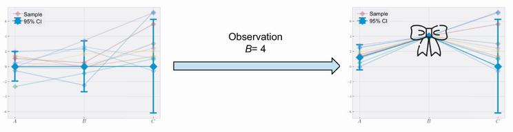
Use the knot analogy to see conditioning: every posterior sample passes through the observation, so uncertainty vanishes at that point. section 2.2.2

How Bayesian Optimization in Action covers it

How deep it goes

Defines posterior updates and works through Gaussian conditioning effects, but defers the closed-form derivation.

Examples

Illustrates updates with house prices, correlated variables, repeated psychic guesses, and a remote-control search.

What you can do after

Evaluate/understand how relevant observations shift predictions and reduce uncertainty under a Bayesian model.

How it connects

Connects Bayes’ theorem, conditioning, multivariate Gaussian distributions, covariance, and Gaussian processes.

liveBookmanning.com

Read Bayesian Optimization in Action on liveBook Get the book at manning.com

Also explained in

• 

  liveBookmanning.com
  Grokking Machine LearningA posterior probability is the probability assigned to an event or hypothesis after incorporating observed evidence.
• 

  liveBookmanning.com
  Math and Architectures of Deep LearningThe updated distribution over model parameters after combining prior and likelihood.
• 

  liveBookmanning.com
  Fabulous Adventures in Data Structures and AlgorithmsA posterior distribution is a probability distribution representing beliefs about an unknown quantity after incorporating observed evidence.
• 

  liveBookmanning.com
  Build a Robo-Advisor with Python (From Scratch)A posterior distribution is a probability distribution representing updated beliefs about an unknown quantity after incorporating data or observations.
• 

  liveBookmanning.com
  AI-Powered SearchA posterior distribution is a probability distribution representing an updated belief after incorporating observations into a prior distribution.
• 

  liveBookmanning.com
  Machine Learning Algorithms in DepthA posterior distribution is the probability distribution of unknown quantities after incorporating observed data into prior beliefs.
• 

  liveBookmanning.com
  Causal AIA posterior distribution is the conditional probability distribution of unknown quantities given observed data and prior assumptions.

Compare how 8 books explain posterior probability →

Related concepts

• bayesian statisticsproduced by · Bayesian statistics is a framework for statistical inference that combines prior probability distributions with observed-data likelihoods to update probabilities over hypotheses or unknown quantities.
• prior probabilityproduced by · A prior probability distribution represents beliefs or assumptions about an unknown quantity before relevant observations or evidence are incorporated.
• Bayes' theoremproduced by · Bayes' theorem is a probability rule that expresses a conditional probability in terms of a prior probability, a likelihood, and the evidence.
• markov chain monte carloused by · Markov chain Monte Carlo is a family of sampling algorithms that generate samples using a Markov chain whose stationary or limiting distribution is a target probability distribution.
• fully bayes parameter estimationproduced by · Fully Bayesian parameter estimation combines a prior distribution with observed-data likelihood to produce a posterior distribution over unknown parameters.

This explainer was generated by Manning's knowledge graph from the text of Bayesian Optimization in Action. The section links point to the parts of the book it draws on.