A principal component is a data point’s coordinate after projection onto a principal axis. The first principal axis is the covariance matrix eigenvector with the largest eigenvalue, because it captures the direction of maximum variance. Components along later orthogonal axes capture successively smaller variance. section 4.4.1
For a unit direction l̂ and data vector x, the projected coordinate is l̂ᵀx. Collecting these coordinates gives a lower-dimensional representation. Discarding coordinates associated with small eigenvalues removes directions with little spread and usually little information. section 4.4.1 section 4.4.2
Principal components connect geometric structure, storage, and computation:
- Represent the dominant directions of a dataset; their variances equal the corresponding covariance-matrix eigenvalues. section 4.4.1
- Reduce dimensionality by retaining components with the largest principal values and removing small-variance directions. section 4.4.2
- Support compression by storing projections onto only the first few principal axes. section 4.4.5
- Represent topics in latent semantic analysis, where document-vector directions with high variance expose correlated vocabulary. section 4.6.2
Correlated document features
Construct 500 document vectors with x₁ approximately twice x₀ and x₂ varying only slightly. SVD finds a dominant component along the correlated x₀–x₁ direction; the small third singular value indicates that the x₂ variation can be ignored. section 4.6.4
Figure 4.3 Dimensionality reduction via PCA. Original data points are shown with filled little circles, and hollow circles represent lower-dimensional representations.
|
(a) Dimensionality reduction from 2D to 1D |
|
(b) Dimensionality reduction from 3D to 2D |
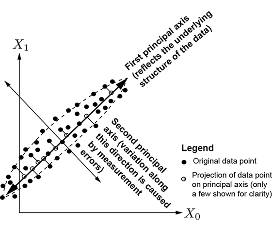
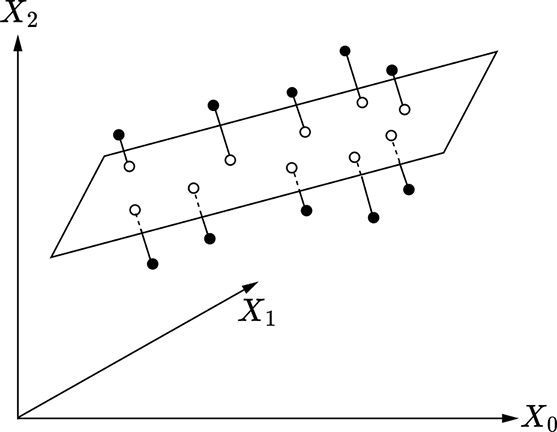
Compare 2D-to-1D and 3D-to-2D projections to see how dominant principal components preserve structure while removing small orthogonal variations. section 4.4.2




