A principal value is the variance measured along a principal axis found by PCA. Each value pairs with a principal vector: the largest value marks maximum spread, and subsequent values mark orthogonal directions with decreasing variance. section 14.4 section 4.4.1
Small principal values identify directions containing little variation. Removing their corresponding principal components can reduce dimensionality, suppress likely noise, and preserve most information with low reconstruction loss. section 14.4 section 4.4.2
Use principal values to interpret PCA representations:
- Rank principal axes by their values; larger values represent directions of greater data spread. section 4.4.1
- Keep axes with comparatively large values and discard axes with small values when the resulting information loss is acceptable. section 4.4.2
- Store projections onto the leading axes to reduce the number of components required for data compression. section 4.4.5
A 3D dataset near a plane
For points clustered around the X0 = X2 plane, the two larger principal values correspond to in-plane directions. The much smaller third value corresponds to the normal direction, so setting that component to zero produces a 2D representation with little information loss. section 14.4
Figure 14.3 The original 3D data in figure 14.3a shows high correlation: points are clustered around the X0 = X2 plane. The first principal component corresponds to the direction of maximum variance. The last (third) principal reduced to a 2D latent vector.
|
(a) Original 3D data |
|
(b) Lower-dimensional 2D representation obtained by setting the third principal value to zero |
|
(c) The principal vectors of the original data. The third principal vector is normal to X0 = X2 plane; the other two are in-plane. |
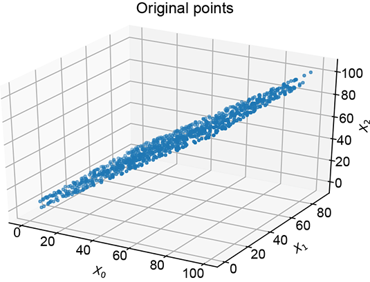
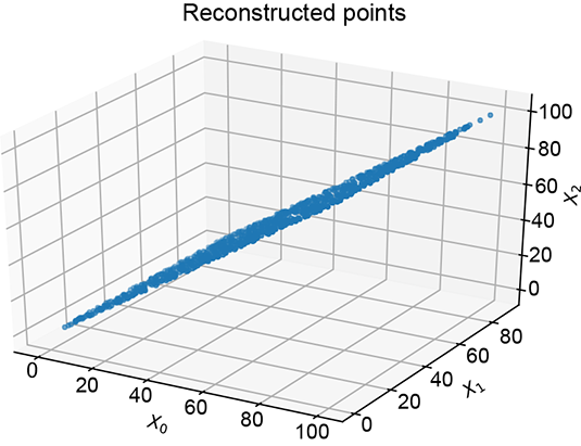
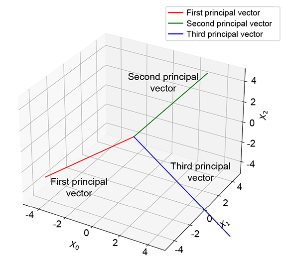
Compare the original 3D points, their 2D projection after zeroing the smallest principal value, and the three principal vectors. section 14.4
