A probability mass function (PMF) gives the actual probability of each possible value of a discrete random variable. Written P(X = x), it assigns a nonnegative probability to every possible value x, and those probabilities sum to 1. Its formula depends on the distribution being modeled; there is no single PMF for all discrete variables. section 2.4.2
A PMF answers a different question from a probability density function (PDF): a PMF gives the probability of one specific discrete value, while a PDF describes relative likelihood across a continuous range. To find the probability of several discrete outcomes, add their PMF values. A discrete cumulative distribution function (CDF) likewise rises in steps as outcome probabilities accumulate. section 2.4
Counting outcomes for two dice
Let X be the total on two fair six-sided dice. There are 36 possible rolls. Only one totals 2, so P(X = 2) = 1/36 ≈ 0.0278; two total 3, so P(X = 3) = 2/36 ≈ 0.0556. The probabilities differ because the totals have different numbers of ways to occur. section 2.4.2
Figure 2.4 The PMF for rolling a pair of six-sided dice, where the discrete random variable and its possible values, which are equal to the whole numbers between 2 and 12, are plotted along the x axis, and their respective probabilities of occurrence are plotted along the y axis. The y axis represents their actual probabilities, not their relative likelihood of occurrence. All probabilities are equal to or greater than zero.
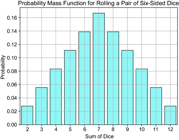
Inspect how the probability changes across possible two-dice totals from 2 through 12; the vertical axis shows actual probabilities. section 2.4.2
Choose the PMF that matches how the outcomes arise:
- Discrete uniform: every value in a finite range has the same probability. For integer bounds a through b, there are b − a + 1 values, each with probability 1/(b − a + 1). A fair die therefore assigns 1/6 to each face. section 3.1.3 section 2.4
- Binomial: calculate the probability of k successes in a fixed number of independent trials, each with the same success probability. For example, `scipy.stats.binom.pmf(7, 20, 0.2)` returns about 0.05455. section 3.1.2
- Poisson: calculate the probability of k events in a fixed interval given an average rate λ. For example, `scipy.stats.poisson.pmf(4, 2)` returns about 0.09022. section 3.1.4
Before interpreting a computed probability, check that the chosen distribution fits the situation. Equal probabilities justify a discrete uniform model; binomial probabilities depend on its repeated-trial assumptions; a Poisson calculation depends on an average event rate for a fixed interval. section 3.1.2 section 3.1.4


