Quantum measurement extracts classical information from a quantum state. It is the final readout step of a typical quantum algorithm: prepare a state, evolve it, then measure to obtain an answer. Unlike classical observation, measurement is probabilistic for superpositions, returns limited information, and can change the state. section 4.0
By default, measurement is in the computational basis. Measuring α|0⟩ + β|1⟩ returns 0 with probability α² and 1 with probability β²; for multiple qubits, each basis-string outcome has probability equal to the squared amplitude of that basis state. A basis state is returned with certainty. section 4.1.1
Figure 4.1 Any quantum algorithm can be broken down into several steps: prepare the initial state, evolve it following the algorithm, and measure the end state to get the result. In this chapter, we’ll learn to work with the final step, measuring the state of the system to extract information about it.
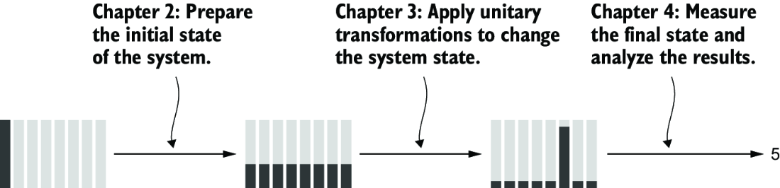
Use this workflow diagram to place measurement within the prepare–evolve–measure structure of a quantum algorithm. section 4.0
Measurement supports several practical readout tasks:
- Identify a known basis state by measuring its qubits and interpreting the resulting bit string. section 4.1
- Distinguish designated superposition states when their possible basis-state outcomes do not overlap. section 4.2.1
- Extract partial information, such as parity, through a joint measurement while preserving a relevant superposition. section 4.6
Recognizing a three-qubit state
For a promised input drawn from four superpositions with disjoint basis states, measure all three qubits and map outcomes to the unique state containing that outcome. For example, 000 or 111 identifies (|000⟩ + |111⟩)/√2. section 4.2.1
Repeated hardware measurements can estimate outcome probabilities and amplitudes, but cannot recover relative phase and may be biased by noise. For small systems, noiseless simulators can expose an internal classical state representation for inspection instead of relying only on measurement samples. section 2.2
Measurement design determines what can be learned. Orthogonal states can be distinguished perfectly with an appropriate procedure, potentially in a noncomputational basis; nonorthogonal states cannot. Multiple copies enable more detailed analysis through quantum state tomography. section 4.9