A quantum operation changes a quantum state as required by an algorithm. In the common prepare–evolve–measure workflow, the operation supplies the evolution step: algorithms describe a transformation, programs express it with gates and language constructs, and hardware executes native instructions. section 3.0 section 3.13
Figure 3.2 The transformation the quantum state undergoes following a quantum algorithm is typically broken down into simpler building blocks. First, the whole algorithm is expressed as a sequence of operations described in terms of the input parameters of the problem. These operations are further represented as sequences of primitives provided by the high-level programming language used to implement the algorithm. Finally, to execute the algorithm on a quantum device, programming language primitives have to be expressed as sequences of low-level instructions that are natively available on this device.
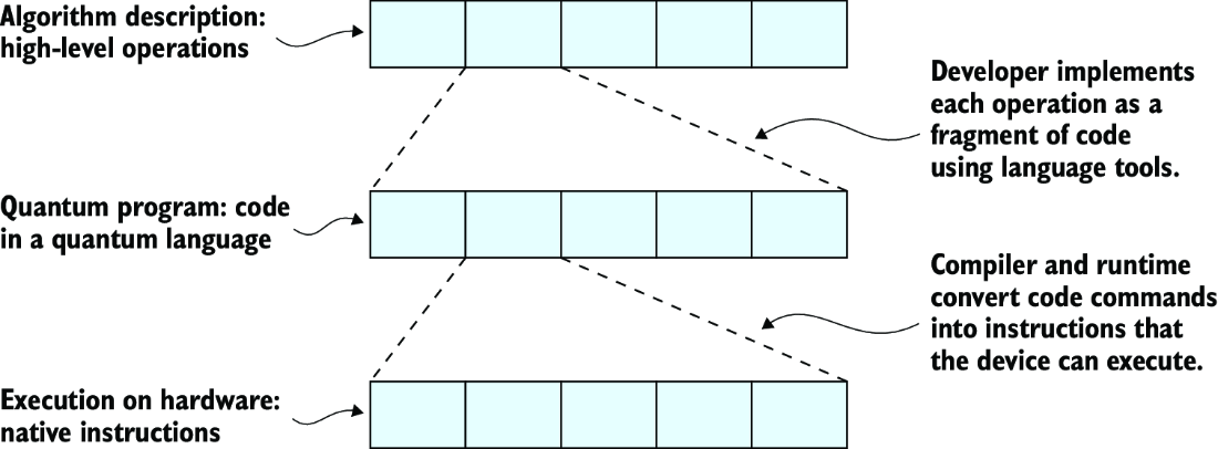
Follow how one transformation is refined from problem-level operations to programming primitives and device-native instructions. section 3.0
Implementing a unitary operation means converting its matrix description into a gate sequence with the same transformation. A single-qubit unitary given by four matrix entries is a foundational implementation task; larger unitaries can be built recursively by decomposing matrices and using controlled operations on fewer qubits. section 3.1 section 3.13
Treat an implementation as a testable artifact:
- Validate that the operation implements the expected matrix with unit tests, simulators, and specialized tools. section 3.3
- Inspect an implemented matrix through simulator access to quantum states during execution. section 3.13
- Analyze an unknown operation by choosing initial states, applying it or variants, measuring results, and repeating or varying runs when statistics require it. section 5.0
Reversibly encode a classical function
Extend a one-bit function to F(x,y) = (x, y ⊕ f(x)) so the input information is preserved. For f(x) = 1, apply X to the second qubit; for f(x) = x, use CNOT with x as control. Linearity then defines the gate’s action on superposition inputs. section 6.2.1
Table 6.1 Single-bit functions and their reversible two-bit extensions
| Function \(f(x)\) | Extended function \(F(x, y)\) | Extended input | Extended output |
| \(f(x) = 1\) | \(F(x, y) = (x, y \oplus 1)\) | \((0, 0)\) | \((0, 1)\) |
| \((0, 1)\) | \((0, 0)\) | ||
| \((1, 0)\) | \((1, 1)\) | ||
| \((1, 1)\) | \((1, 0)\) | ||
| \(f(x) = x\) | \(F(x, y) = (x, y \oplus x)\) | \((0, 0)\) | \((0, 0)\) |
| \((0, 1)\) | \((0, 1)\) | ||
| \((1, 0)\) | \((1, 1)\) | ||
| \((1, 1)\) | \((1, 0)\) |
Compare the input–output mappings for reversible two-bit extensions of constant and identity single-bit functions. section 6.2.1