A receptive field is the region of the original input that can influence one output pixel or voxel. A convolution starts with a small neighborhood, but stacking layers lets later outputs draw on a wider area. section 8.2.3 section 13.4.1
Trace one output pixel backward
Start with an 8 × 8 image. Apply a 3 × 3 convolution, halve the image with max pooling, then apply another 3 × 3 convolution. One output of the second convolution depends on several pooled values, each representing an area of the first convolution’s output. Tracing those dependencies back gives an 8 × 8 receptive field away from the boundary. At a padded corner, only a 7 × 7 region of actual input pixels contributes. section 8.2.3
The same idea applies to volumes. One 3 × 3 × 3 convolution sees 3 × 3 × 3 input voxels; two stacked convolutions give an output voxel an effective 5 × 5 × 5 receptive field. Stacking these smaller kernels uses fewer parameters than one 5 × 5 × 5 convolution. A following max-pooling layer widens the region represented by its output again. section 13.4.1
Figure 8.10 More convolutions by hand, showing the effect of stacking convolutions and downsampling: a large cross is highlighted using two small, cross-shaped kernels and max pooling
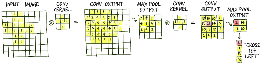
Follow the small convolutions and downsampling to see how a later output responds to a larger pattern. section 8.2.3

