Stochastic gradient descent (SGD) minimizes a loss by repeatedly estimating its gradient from a randomly selected subset of training examples, then moving the parameters in the opposite direction. Using a mini-batch of size m avoids computing every update from the full dataset. section 10.4
Let θ be the model parameters, L the loss, and εₖ the learning rate at iteration k. For examples (xᵢ, yᵢ) in a mini-batch, estimate gₖ = (1/m)∑ᵢ ∇θ L(f(xᵢ; θₖ), yᵢ), then update θₖ₊₁ = θₖ − εₖgₖ. The gradient gives the direction of increasing loss; the minus sign makes the update a minimization step. A larger εₖ moves farther on each update but can miss an optimum. A smaller one may make training unnecessarily slow. section 10.4
For a training loop, the key choices are:
- Sample a mini-batch, compute its loss gradient, and update the parameters. Repeat over iterations. section 10.4
- Choose a learning-rate schedule. One practical starting value is 10⁻³, followed by reductions as training proceeds; the learning rate may change with iteration. section 10.4
- Consider momentum when successive gradients point in similar directions: it carries an exponentially decaying average of earlier gradients into later updates. Nesterov momentum instead evaluates the gradient after applying the current velocity. section 10.4
Perceptron updates as gradient-based training
For a labeled example, define its margin as zᵢ = yᵢ(θ·xᵢ + θ₀). Hinge loss penalizes insufficient margin. Its piecewise-linear gradient is zero when zᵢ > 1 and gives an update direction when zᵢ ≤ 1; at zᵢ = 1, the max operation is not differentiable, so a subgradient is used. A perceptron implementation samples training examples and updates after a classification error. This connects the classifier’s update rule to stochastic gradient-based loss minimization without making a full-dataset gradient calculation at every step. section 5.2
Figure 10.13 Cross-entropy loss and validation accuracy of LeNet trained on cifar100 using different optimizers
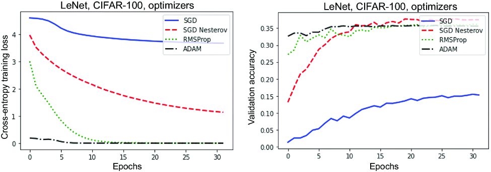
Compare cross-entropy loss and validation accuracy when LeNet is trained on CIFAR-100 with different optimizers; the plot makes optimizer choice a measurable training decision. section 10.4











