Single-world intervention graph

As explained in Causal AI

A single-world intervention graph is a causal graph formed by splitting intervention nodes to represent counterfactual variables under a single-world assumption.

To ask whether a subscriber would respond differently under another recommendation policy, causal analysis must represent both the observed policy and its intervention. A single-world intervention graph (SWIG) does this by splitting intervention nodes and annotating downstream variables with intervention values. section 10.7.3

A SWIG starts with a causal directed acyclic graph and applies node-splitting surgery for each intervention. The original node keeps its parents but loses its children; a new node represents the fixed intervention value. Every downstream node inherits that intervention as a subscript. section 10.7.3

Construct a SWIG as follows:

• Split the target node for an intervention such as do(T = −t). section 10.7.3
• Retain the original node’s parents and redirect its former children to the intervention-value node. section 10.7.3
• Subscript every downstream variable with the intervention value, such as W_T=−t and A_T=−t. section 10.7.3
• Repeat the operation for additional interventions; variables inherit all relevant upstream intervention subscripts. section 10.7.3

Figure 10.20 The intervention operator for a SWIG is the node-splitting operation.

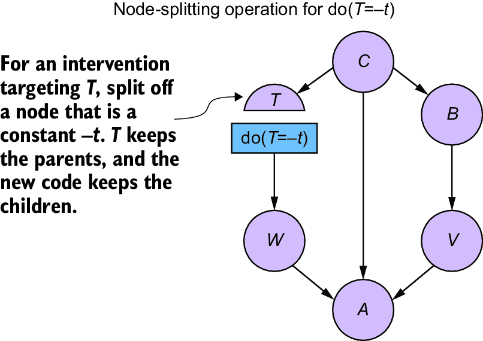
Use the intervention-surgery sequence to inspect how a natural variable and its fixed intervention value coexist in the graph. section 10.7.3

Unlike a parallel-world representation, a SWIG admits d-separation, allowing graphical identification of counterfactual quantities. For example, estimating the effect of treatment on the treated can use confounder C: d-separation permits replacing the treated counterfactual conditional with an observed conditional, while consistency maps the counterfactual outcome to A. section 10.7.4 section 10.10

The construction depends on a single-world assumption: an intervention can be applied while the variable’s natural value remains knowable and unchanged by intervention side effects. This narrows the counterfactual queries available, but supports experimental validation. section 10.7.5

Recommendation-policy counterfactual

Suppose a subscriber naturally receives policy +t, but the system is forced to use −t. A SWIG represents the natural policy value, the intervention value, and downstream outcomes such as A_T=−t, enabling identification under the stated assumptions. section 10.7.5 section 10.7.4

How Causal AI covers it

How deep it goes

Explains node splitting, subscript inheritance, ETT identification, and assumptions, while deferring broader nonidentified counterfactual queries.

Examples

Uses Netflix recommendation policies, treatment-effect-on-the-treated notation, node-splitting figures, and downstream counterfactual variables.

What it assumes

Assumes causal DAGs, interventions, conditional independence, and probability rules while introducing SWIG construction and the single-world assumption.

What you can do after

Evaluate identified counterfactual quantities using SWIGs, d-separation, and probabilistic inference implemented through Pyro.

How it connects

Connects causal DAGs, counterfactual graphs, d-separation, ignorability, consistency, do-calculus, and probabilistic inference.

liveBookmanning.com

Read Causal AI on liveBook Get the book at manning.com

Related concepts

• counterfactual graphalternative to · A counterfactual graph is a graph formed by collapsing equivalent nodes across the intervention worlds of a parallel world graph while retaining nodes relevant to a counterfactual query.
• do functionimplemented by · A do function is an API operation that applies a causal intervention by setting a sampled variable to a specified value while preserving its downstream effects.
• node-splitting operationuses · A node-splitting operation replaces an intervention node in a causal graph with separate components representing its intervened and natural values.
• d-separationuses · D-separation is a graphical criterion for determining whether a conditioning set blocks all relevant paths between variables in a graph, implying conditional independence under the graph’s assumptions.
• causal identificationuses · Causal identification is the process of determining whether a causal quantity can be uniquely computed from available observational or interventional information and model assumptions.
• counterfactual outcomehas part · A counterfactual outcome is a hypothetical result that would have occurred under a condition, action, or intervention different from the one observed.

This explainer was generated by Manning's knowledge graph from the text of Causal AI. The section links point to the parts of the book it draws on.