Suppose you want to estimate the true atmospheric CO₂ concentration each year, but measurements are noisy. A state transition model describes how that hidden concentration can change from one year to the next. An observation model separately describes how measurements relate to it. section 9.2
A simple choice is a random walk: xᵢ₊₁ = xᵢ + ε. The next state is expected to equal the current state, while ε allows random changes. Here ε has a zero-mean Gaussian distribution; its variance σ² controls how widely the next state can vary. Small changes are more likely than large ones. section 9.6
Choosing and checking the transition variance
One starting choice is to load the CO₂ measurements with NumPy, compute year-to-year differences with np.diff(y), and set S = np.var(diffs). This uses the data to choose a noise variance. If the filter then adjusts too little to new measurements, increasing the transition variance makes its predictions less certain and can help it track the data. section 9.6 section 9.10
The transition model supplies a filter’s prediction before the next measurement arrives. The observation model helps update that prediction afterward. A random walk has a limitation: without an explicit trend, its long-range forecast has a flat mean even as uncertainty grows. section 9.3 section 9.10
To represent a persistent rise, the hidden state can include both concentration level ℓ and slope s. Then ℓᵢ₊₁ = ℓᵢ + sᵢ + ε, while sᵢ₊₁ = sᵢ + e. The slope carries the trend forward, and both transitions allow noise. section 9.12
Figure 9.3 A diagram of a state space model, which includes an unknown latent space 𝑥ᵢ that evolves over time, and the observation model, which describes the relationship between the latent state and observed data 𝑦ᵢ at each time step.
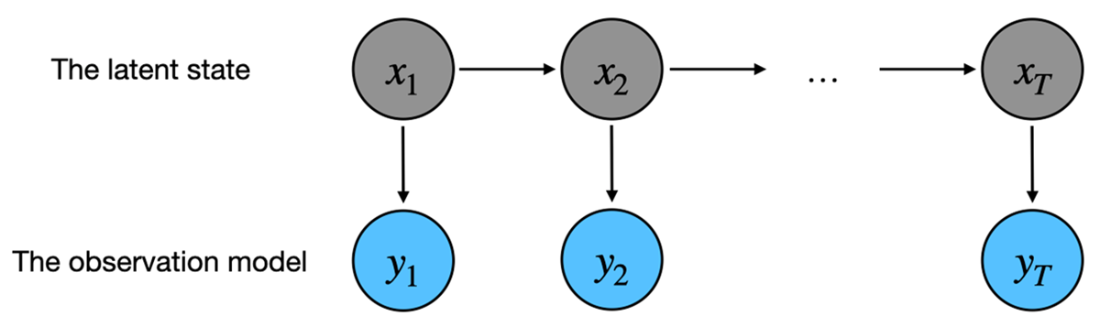
The diagram separates the evolving hidden state from the measurements generated at each time step. section 9.2
