Support vector machine

As explained in Grokking Machine Learning

A model that separates classes or fits targets using an optimized margin and support vectors.

Suppose several lines can separate cats from dogs. Which line is safest? A support vector machine (SVM) chooses a boundary with the greatest possible space on both sides, making it more robust when points shift slightly. section 11.0

An SVM uses a central boundary and two parallel lines around it. Training balances two goals: classify points correctly and keep the parallel lines widely separated. The resulting boundary may be a line, plane, or higher-dimensional hyperplane. section 11.0 section 11.1

The training objective works as follows:

• Represent the central boundary as w1x1 + w2x2 + b = 0, then place parallel boundaries at values 1 and –1. section 11.1
• Measure classification error from points assigned to the wrong side of the boundaries. section 11.1
• Add a distance-related penalty so boundaries that are too close become less attractive. section 11.1
• Use C to decide how strongly correct classification outweighs a widely spaced boundary: small C tolerates mistakes, while large C emphasizes correct classification. section 11.1 section 11.2

A linear SVM cannot fit a dataset such as XOR because the classes are not linearly separable. The kernel method addresses this by embedding the data in a higher-dimensional space, where a linear boundary may separate it. Polynomial kernels can form circles, parabolas, and hyperbolas; RBF kernels can form more complex curved regions. section 11.4 section 11.5

Training a linear SVM

With Scikit-Learn, import SVC, create SVC(kernel='linear'), and fit it to feature and label data. A sample model reaches 0.933 accuracy. Comparing C=0.01 with C=100 shows the practical trade-off: the smaller value gives a wider-spaced boundary with mistakes, while the larger value avoids mistakes but may place the boundary close to points. section 11.2

Figure 11.2 We draw our classifier as two parallel lines, as far apart from each other as possible. We can see that classifier 2 is the one where the parallel lines are the farthest away from each other. This means that the middle line in classifier 2 is the one best located between the points.

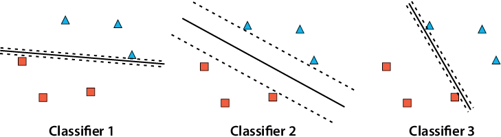
Use the parallel-boundary diagram to compare margins visually and identify why the widest spacing is preferred. section 11.0

How Grokking Machine Learning covers it

How deep it goes

Explains geometry, error terms, C, Scikit-Learn coding, and kernels, while stopping short of a full optimization derivation.

Examples

Uses competing separating lines, parallel margin diagrams, linear.csv, C comparisons, and the XOR dataset.

What it assumes

Assumes familiarity with perceptrons and linear classifiers while developing the SVM objective and kernel intuition from geometric examples.

What you can do after

Apply SVMs via Scikit-Learn, tune C, compare margins, and select kernels for nonlinear classification.

How it connects

Connects SVMs to perceptrons, linear classifiers, error functions, Scikit-Learn, and the kernel method.

liveBookmanning.com

Read Grokking Machine Learning on liveBook Get the book at manning.com

Also explained in

• 

  liveBookmanning.com
  Sutskever's ListA support vector machine is a supervised learning model that determines decision boundaries using maximum-margin principles.
• 

  liveBookmanning.com
  Machine Learning Algorithms in DepthA supervised learning model that separates classes by selecting a decision boundary with a large margin, optionally using a kernel for nonlinear separation.
• 

  liveBookmanning.com
  Data-Driven CybersecurityA support vector machine is a supervised-learning model that separates classes or predicts values by constructing a boundary based on support vectors.
• 

  liveBookmanning.com
  Ensemble Methods for Machine LearningA support vector machine is a supervised learning model that finds a maximum-margin separating function, optionally using kernels to represent nonlinear decision boundaries.

Compare how 5 books explain support vector machine →

Related concepts

• kernel functionuses · A kernel function is a mathematical function that measures similarity between pairs of inputs, often representing an inner product in an implicit feature space.
• anomaly detectionuses · Anomaly detection is the identification of observations, events, or behaviors that substantially deviate from expected patterns or a normal baseline.
• classifierkind of · A classifier is a predictive computational model that assigns inputs to one or more discrete classes or categories.
• convex optimizationuses · Convex optimization is the minimization or maximization of a convex or concave objective over a convex feasible set, a structure that permits global optimality guarantees.

This explainer was generated by Manning's knowledge graph from the text of Grokking Machine Learning. The section links point to the parts of the book it draws on.