Surface

As explained in Geometry for Programmers

A surface is a two-dimensional geometric set embedded in or describing a space.

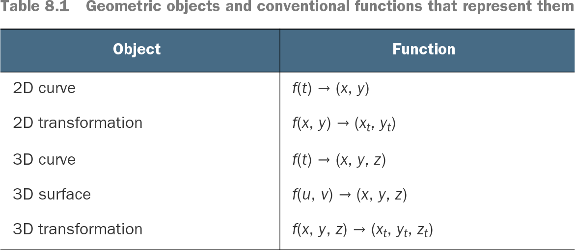
A surface is a two-dimensional geometric object in 3D, usefully modeled as a transformation of a plane. Rather than treating it only as a graph z = f(x, y), describe each point with two parameters: f(u, v) → (x, y, z). This view can represent shapes such as spheres and cylinders that ordinary function graphs cannot close. section 8.2.1 section 8.2.3

Table 8.1 Geometric objects and conventional functions that represent them (view table figure)

Object	Function
2D curve	f(t) → (x, y)
2D transformation	f(x, y) → (xt, yt)
3D curve	f(t) → (x, y, z)
3D surface	f(u, v) → (x, y, z)
3D transformation	f(x, y, z) → (xt, yt, zt)

Compare a surface’s two-parameter point function with curve and transformation functions. The extra input parameter is what lets a surface span an area rather than trace a line. section 8.2.1

Think of the construction as bending an infinite sheet of metal with a point transformation. Start from points on a plane, supply their two coordinates, and compute transformed x, y, and z coordinates. The parameter domain need not literally be the x-y plane; u and v conventionally name its coordinates. section 8.2.1

Choose a representation according to the job:

• Use smooth parametric surface pieces when CAD or CAE needs surface smoothness; their boundaries live in UV space. section 11.0
• Use triangle meshes when rendering speed matters, including games, augmented reality, virtual reality, and computer-generated imagery. section 11.0
• Convert smooth surfaces to triangles and then to stacked contours in a 3D-printing pipeline; printable manifold meshes can avoid corrective postprocessing. section 1.0

From a square to a closed model

A closed surface comes from transforming a specific piece of a plane rather than the entire plane. A standard square provides a practical parameter domain, such as [0..1] × [0..1], for building a bounded surface patch; a mushroom mesh can be generated by evaluating f(u, v) → (x, y, z) into vertices and triangles. section 8.2.3 section 11.0

Surface modeling reuses familiar ideas rather than requiring wholly new 3D mathematics. Parametric curves, transformations, polynomial interpolation, and spatial interpolation all extend to surface construction and deformation. Grid-aligned interpolation data can be decomposed into simpler single-variable computations for faster evaluation. section 8.0 section 8.6

Figure 11.1 A torus described as a smooth surface (left) and as a triangle mesh of ~10,000 triangles (right)

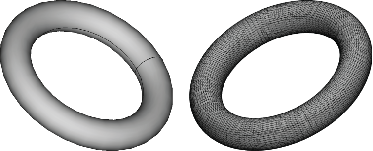
A torus makes the precision-versus-size trade-off visible: one model is a smooth surface, while the other approximates it with roughly 10,000 triangles. section 11.0

How Geometry for Programmers covers it

How deep it goes

Defines surfaces as plane transformations, derives parametric notation, and connects construction to interpolation, deformation, meshes, and boundary representations.

Examples

Uses bent-page correction, a mushroom triangle mesh, a torus comparison, and smooth-model-to-contour 3D-printing conversion.

What it assumes

Builds on coordinate-based geometry, transformations, parametric curves, derivatives, and polynomials while presenting 3D surface construction as an extension.

What you can do after

Build it from scratch as a parametric plane transformation and choose smooth patches or triangle meshes for practical constraints.

How it connects

Connects parametric curves, transformations, polynomial interpolation, spatial interpolation, triangle meshes, boundary representation, and signed distance functions.

liveBookmanning.com

Read Geometry for Programmers on liveBook Get the book at manning.com

Related concepts

• surface of revolutionincludes · A surface of revolution is a surface generated by rotating a curve around an axis.
• pointhas part · A point is a zero-dimensional location in a geometric or coordinate space represented by an ordered set of coordinate values.
• manifoldkind of · A manifold is a mathematical space that locally resembles Euclidean space, although its global geometry or topology may be more complex.
• triangleimplemented by · A triangle is a polygon bounded by three line segments joining three noncollinear vertices.
• planeuses · A plane is a flat two-dimensional geometric surface extending indefinitely in two independent directions.

This explainer was generated by Manning's knowledge graph from the text of Geometry for Programmers. The section links point to the parts of the book it draws on.