A symmetric quadratic Bézier curve draws a curved edge between two endpoints while constraining its control point to remain equidistant from both. The control point therefore lies on the perpendicular bisector of the endpoint segment, so the curve can be represented by the endpoints and one signed distance d from their connecting line. Positive and negative d place the curve on opposite sides of the segment. section 16.1.2
This restriction provides useful geometric properties:
- The curve is a section of a parabola, and its control point can be stored with one real value describing its distance from the endpoint line. section 15.4.4
- The tangent parallel to the endpoint segment lies halfway between that segment and the control point, at distance d/2. section 15.4.4
- For curve intersections, interval subdivision uses axis-parallel tangents to split each curve into monotonic sections, then approximates sufficiently small sections with segments. section 15.4.4
Curved graph edges
Represent an edge between vertices u and v with the endpoints plus d. Restricting the magnitude of d to roughly the endpoint distance limits extreme shapes while preserving a controllable choice of curvature; negative d flips the curve to the opposite side of uv. section 16.1.2
Figure 15.23 A quadratic Bézier curve where the control point lies at the same distance from the endpoints. The tangent to the curve parallel to the segment sE is at a distance of d/2 from that segment, where d is the distance of point C from segment sE.
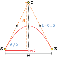
Use the geometric diagram to inspect the perpendicular control-point relationship and the tangent located at d/2. section 15.4.4
Figure 15.26 The interval subdivision method used to check intersections between two symmetric, quadratic Bézier curves (A). (B) Compute the bounding boxes using what we know about the curve’s tangents at apex. Here, they overlap. (C) We thus need to move forward, computing the tangents to the curve parallel to the axes, and use them as pivot points at which we can split the curves. Each section is now monotonic and can be interpolated with a segment. Each pair of sections from the two curves will at most cross in one point. (D) For each section in curve C1, compute the intersections using only the overlapping sections in curve C2 (then sum the results for each of the three cases). (E) We can split each section further by halving it. Only some sub-sections will still overlap, and we can iterate steps (D-E) until they become small enough that the error in approximating a curve with a segment is within a given threshold.
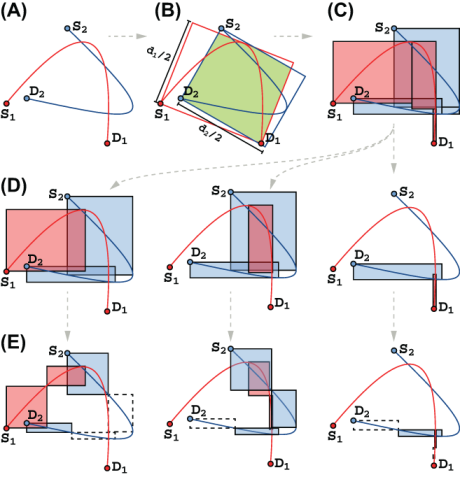
Use the intersection diagram to follow bounding-box checks, monotonic subdivision, overlapping-section tests, and refinement by halving. section 15.4.4
