Parabola

As explained in Experimentation for Engineers

A quadratic curve whose graph can represent a response changing with one parameter and having an interior maximum or minimum.

A parabola is a quadratic curve used as a local surrogate for how a business metric changes with one continuous parameter. With three nearby measurements, its hump can place a maximum at an unmeasured interior value, unlike a line fitted through only two points, whose maximum stays at an endpoint. section 4.1.1

Use the curve locally rather than as a global claim about the response. A metric can have an arbitrary overall shape, but near a maximum it may resemble a parabola; measurements taken too far from that peak can break the approximation. Keeping the three parameter values close limits experiment cost while supporting interpolation. section 4.1.1

Fit and use a parabolic surrogate as follows:

• Choose three nearby values of a continuous, ordered parameter with interior values. section 4.1.1
• Randomize parameter selection and collect replicated measurements at each value; aggregate the resulting metric estimates and their standard errors. section 4.1.2
• Fit ŷ = β0 + β1x + β2x² with linear regression, where x is the parameter and y is the aggregate metric. section 4.1.3
• Evaluate the fitted curve between the measured values and select the parameter yielding its highest interpolated value. section 4.1.3

Choosing a trading threshold

Measure markout profit at thresholds 0.5, 1.0, and 1.5, then fit a parabola through the three aggregate results. Even if 1.0 is the best measured threshold, the fitted curve can estimate a more profitable unmeasured threshold within the 0.5–1.5 range. Because three measurements equal the model’s three parameters, this fit is exact at those points; that does not establish accuracy away from them. section 4.1.2 section 4.1.3

Figure 4.6 Measured values of markout_profit(threshold) and interpolations between them. When we interpolate between only two measured values, shown as filled dots in (a) and (b), the maximum profit occurs at one of the measured values. When a third measured value is added, as in (c) and (d), the maximum profit may occur at an interpolated value, shown as an unfilled dot in (c) and (d). Thus, for interpolation to be useful in estimating an optimum at an unmeasured value of threshold, at least three points must be measured.

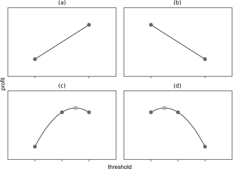
Compare the two-point case, where an endpoint wins, with the three-point case, where the interpolated parabola can peak between observations. section 4.1.1

How Experimentation for Engineers covers it

How deep it goes

Works through three-point quadratic regression and interpolation, while limiting validity to a local range near a maximum.

Examples

Uses simulated markout profit at thresholds 0.5, 1.0, and 1.5 with error-barred aggregate measurements.

What it assumes

Defers a short introduction to linear regression to an appendix while defining the quadratic model terms.

What you can do after

Apply it via linear regression to interpolate a local profit curve and choose its maximizing threshold.

How it connects

Connects response surface methodology with interpolation, linear regression, continuous parameters, and experimental randomization.

liveBookmanning.com

Read Experimentation for Engineers on liveBook Get the book at manning.com

Related concepts

• polynomial functionkind of · A polynomial function is a function expressible as a finite sum of constant multiples of nonnegative integer powers of one or more variables.
• interpolationused by · Interpolation is the estimation or construction of values or representations between known points according to an assumed relationship or specified rule.
• symmetric quadratic Bézier curvehas part · A symmetric quadratic Bézier curve is a quadratic Bézier curve whose control point is equidistant from its two endpoints.
• response surface methodologyuses · A statistical optimization methodology that models a response as a function of controllable factors to identify promising settings.

This explainer was generated by Manning's knowledge graph from the text of Experimentation for Engineers. The section links point to the parts of the book it draws on.