Ternary quantization maps each weight to {−1, 0, +1}: a weight votes positive, votes negative, or abstains. Multiply-accumulate then reduces to addition and subtraction. The information-theoretic cost is about 1.58 bits per weight; packing five ternary values per byte gives an effective 1.6 bits. section 8.5
The tradeoff is sparse representational coverage near zero. After absmax normalization, values not near ±1 can round to zero or the wrong sign; a scale factor cannot repair that error. A 7B model could shrink from 3.5 GB in NF4 to roughly 1.4 GB, but only if it survives the compression. section 8.5
Figure 8.17 Representable values in [−1, 1]. Ternary (top row) has 3 levels — only the endpoints and zero. NF4 (16 levels) and FP4 E2M1 (15 levels) pack 7 values each into the [−0.3, 0.3] interval where most neural network weights concentrate. INT4 (16 levels) places 4. Ternary places 1. The visual gap between 3 levels and 15–16 is the cost of halving the bit width twice.
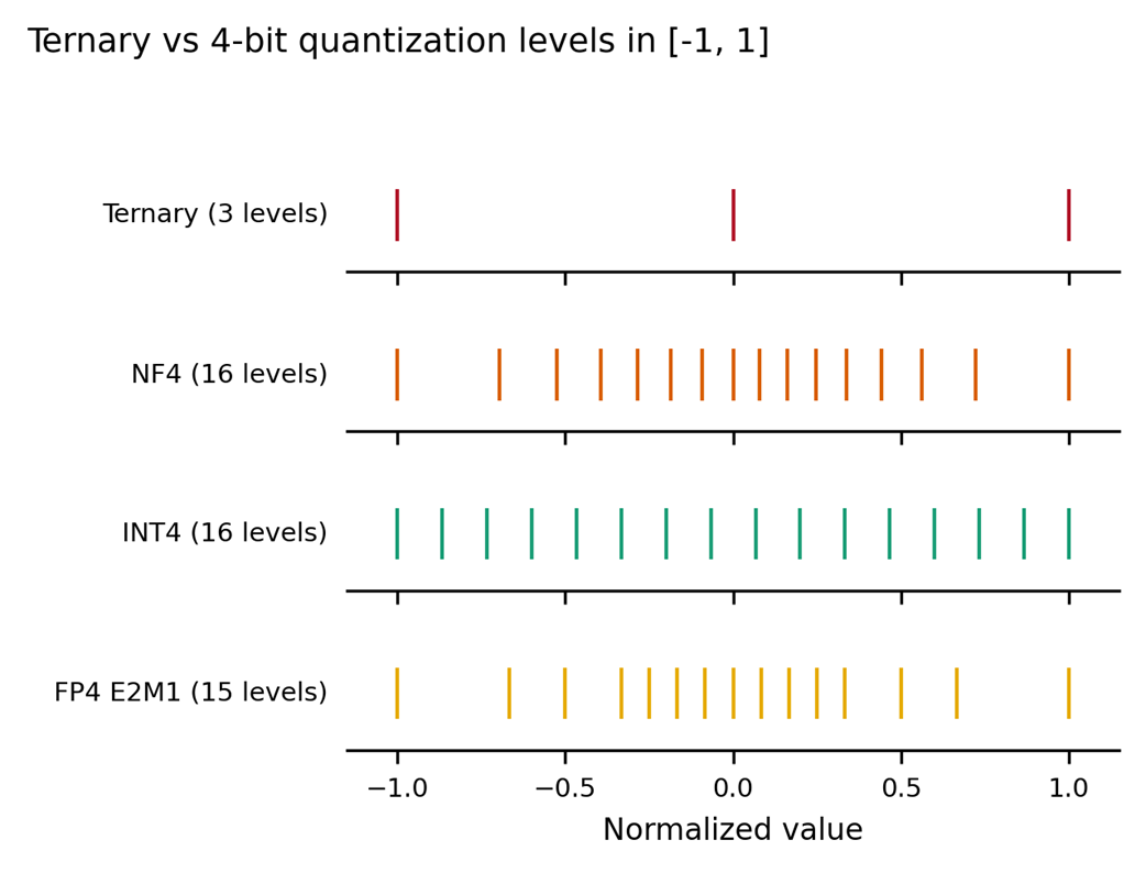
Compare how few values ternary provides near zero against NF4, FP4, and INT4. section 8.5
Post-training ternarization can destroy model quality because the model never adapts to rounding. BitNet b1.58 instead quantizes weights during every training pass and uses a straight-through estimator (STE) to route gradients to full-precision master weights. section 8.5.2
Listing 8.2 Loading Llama-2-7B in NF4 with QLoRA adapters
def weight_quant(w, eps=1e-5):
    scale = 1.0 / w.abs().mean().clamp(min=eps)
    return (w * scale).round().clamp(-1, 1) / scale             #A

def activation_quant(x, eps=1e-5):
    scale = 127.0 / x.abs().amax(dim=-1, keepdim=True).clamp(min=eps)
    return (x * scale).round().clamp(-128, 127) / scale         #B

class BitLinear(nn.Linear):
    def forward(self, x):
        x_q = x + (activation_quant(x) - x).detach()            #C
        w = self.weight
        w_q = w + (weight_quant(w) - w).detach()                 #C
        return F.linear(x_q, w_q, self.bias)
Inspect a BitLinear implementation that quantizes weights and activations while preserving gradient flow. section 8.5.2
Training versus post-hoc rounding
On a toy MLP regression task, BitLinear QAT reaches test MSE 0.0070, versus 0.0052 for FP32; post-hoc ternarization reaches 0.0199. Training with the constraint performs substantially better than imposing it afterward. section 8.5.2