How deeply does LLMs in Production cover training loop?

Explains the loop from batches to gradients and implementation components, then extends into speed-memory tradeoffs without deriving optimization theory.

Training loop in LLMs in Production

A training loop is the repeated process of computing model outputs, evaluating loss, calculating gradients, and updating parameters.

A training loop turns data into parameter updates: initialize the model, process batches, compute predictions and loss, backpropagate gradients, and repeat across epochs. Understanding these steps helps when framework abstractions obscure behavior or production constraints. section 2.2.4 section 5.5

A practical loop typically includes:

Prepare and tokenize data, then divide it into batches. section 5.2.1 section 5.5
Initialize model weights and define the architecture, activation functions, final layer, and loss behavior. section 2.2.4 section 5.5
Run forward propagation to produce predictions, calculate loss, backpropagate gradients, and update parameters. section 2.2.4 section 5.5
Tune batch size and memory-saving methods against speed: accumulation and checkpointing save memory but slow training, while mixed precision favors speed. section 5.4.2 section 5.4.2

From language-model prototype to GPT training

A generative CBoW implementation supplies a complete loop around tokenized Hamlet data, while a GPT implementation builds embeddings, positional embeddings, transformer blocks, normalization, and an output head before training in batches. Character-based tokenization is simple but captures too little linguistic information for strong language modeling. section 2.2.4 section 5.2.1

Listing 2.4 Generative CBoW language model implementation

import nltk
import numpy as np
from utils import get_batches, compute_pca, get_dict
import re
from matplotlib import pyplot

with open("hamlet.txt", "r", encoding="utf-8") as f:
    data = f.read()                              #1

data = re.sub(r"[,!?;-]", ".", data)         #2
data = nltk.word_tokenize(data)
data = [ch.lower() for ch in data if ch.isalpha() or ch == "."]
print("Number of tokens:", len(data), "\n", data[500:515])

fdist = nltk.FreqDist(word for word in data)     #3
print("Size of vocabulary:", len(fdist))
print("Most Frequent Tokens:", fdist.most_common(20))

word2Ind, Ind2word = get_dict(data)     #4
V = len(word2Ind)
print("Size of vocabulary:", V)

print("Index of the word 'king':", word2Ind["king"])
print("Word which has index 2743:", Ind2word[2743])

def initialize_model(N, V, random_seed=1):     #5
    """
    Inputs:
        N: dimension of hidden vector
        V: dimension of vocabulary
        random_seed: seed for consistent results in tests
    Outputs:
        W1, W2, b1, b2: initialized weights and biases
    """
    np.random.seed(random_seed)

    W1 = np.random.rand(N, V)
    W2 = np.random.rand(V, N)
    b1 = np.random.rand(N, 1)
    b2 = np.random.rand(V, 1)

    return W1, W2, b1, b2

def softmax(z):      #6
    """
    Inputs:
        z: output scores from the hidden layer
    Outputs:
        yhat: prediction (estimate of y)
    """
    yhat = np.exp(z) / np.sum(np.exp(z), axis=0)
    return yhat

def forward_prop(x, W1, W2, b1, b2):      #7
    """
    Inputs:
        x: average one-hot vector for the context
        W1,W2,b1,b2: weights and biases to be learned
    Outputs:
        z: output score vector
    """
    h = W1 @ x + b1
    h = np.maximum(0, h)
    z = W2 @ h + b2
    return z, h

def compute_cost(y, yhat, batch_size):     #8
    logprobs = np.multiply(np.log(yhat), y) + np.multiply(
        np.log(1 - yhat), 1 - y
    )
    cost = -1 / batch_size * np.sum(logprobs)
    cost = np.squeeze(cost)
    return cost

def back_prop(x, yhat, y, h, W1, W2, b1, b2, batch_size):    #9
    """
    Inputs:
        x:  average one hot vector for the context
        yhat: prediction (estimate of y)
        y:  target vector
        h:  hidden vector (see eq. 1)
        W1, W2, b1, b2:  weights and biases
        batch_size: batch size
    Outputs:
        grad_W1, grad_W2, grad_b1, grad_b2:  gradients of weights and biases
    """
    l1 = np.dot(W2.T, yhat - y)
    l1 = np.maximum(0, l1)
    grad_W1 = np.dot(l1, x.T) / batch_size
    grad_W2 = np.dot(yhat - y, h.T) / batch_size
    grad_b1 = np.sum(l1, axis=1, keepdims=True) / batch_size
    grad_b2 = np.sum(yhat - y, axis=1, keepdims=True) / batch_size

    return grad_W1, grad_W2, grad_b1, grad_b2

def gradient_descent(data, word2Ind, N, V, num_iters, alpha=0.03):     #10
    """
    This is the gradient_descent function
        Inputs:
            data:      text
            word2Ind:  words to Indices
            N:         dimension of hidden vector
            V:         dimension of vocabulary
            num_iters: number of iterations
        Outputs:
            W1, W2, b1, b2:  updated matrices and biases

        """
        W1, W2, b1, b2 = initialize_model(N, V, random_seed=8855)
        batch_size = 128
        iters = 0
        C = 2
        for x, y in get_batches(data, word2Ind, V, C, batch_size):
            z, h = forward_prop(x, W1, W2, b1, b2)
            yhat = softmax(z)
            cost = compute_cost(y, yhat, batch_size)
            if (iters + 1) % 10 == 0:
                print(f"iters: {iters+1} cost: {cost:.6f}")
            grad_W1, grad_W2, grad_b1, grad_b2 = back_prop(
                x, yhat, y, h, W1, W2, b1, b2, batch_size
            )
            W1 = W1 - alpha * grad_W1
            W2 = W2 - alpha * grad_W2
            b1 = b1 - alpha * grad_b1
            b2 = b2 - alpha * grad_b2
            iters += 1
            if iters == num_iters:
                break
            if iters % 100 == 0:
                alpha *= 0.66

        return W1, W2, b1, b2

C = 2      #11
N = 50
word2Ind, Ind2word = get_dict(data)
V = len(word2Ind)
num_iters = 150
print("Call gradient_descent")
W1, W2, b1, b2 = gradient_descent(data, word2Ind, N, V, num_iters)
# Call gradient descent
# Iters: 10 loss: 0.525015
# Iters: 20 loss: 0.092373
# Iters: 30 loss: 0.050474
# Iters: 40 loss: 0.034724
# Iters: 50 loss: 0.026468
# Iters: 60 loss: 0.021385
# Iters: 70 loss: 0.017941
# Iters: 80 loss: 0.015453
# Iters: 90 loss: 0.012099
# Iters: 100 loss: 0.012099
# Iters: 110 loss: 0.011253
# Iters: 120 loss: 0.010551
# Iters: 130 loss: 0.009932
# Iters: 140 loss: 0.009382
# Iters: 150 loss: 0.008889

Inspect the concrete CBoW implementation, including data preparation, vocabulary construction, model initialization, and the training-loop scaffold. section 2.2.4

Figure 5.2 A simplified version of all the steps necessary to train a language model (large or otherwise) from scratch. You must have data, then define all of the model behavior, and only then proceed to train.

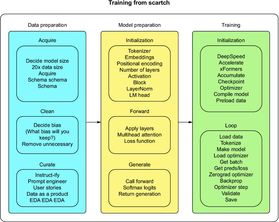
Use the process diagram to follow the dependency from data and model definition to training. section 5.2.1

Table 5.2 Training choices to consider

Method	Improve speed	Improves memory utilization	Difficulty
Batch size choice	Yes	Yes	Easy
Gradient accumulation	No	Yes	Medium
Gradient checkpointing	No	Yes	Medium
Mixed precision	Yes	No	Hard
Optimizer choice	Yes	Yes	Easy
Data preloading	Yes	No	Medium
Compiling	Yes	No	Easy

Compare batch size, accumulation, checkpointing, mixed precision, optimizer choice, preloading, and compilation by speed, memory, and difficulty. section 5.4.2

How LLMs in Production covers it

Also explained in

Related concepts

This explainer was generated by Manning's knowledge graph from the text of LLMs in Production. The section links point to the parts of the book it draws on.