A transition probability gives the chance of moving from a current state to a specified next state. In a Markov chain, that chance depends on the current state, not the sequence of states that came before it. In a Markov decision process, the action taken also helps determine the distribution of possible next states. These probabilities make uncertain moves usable in search and planning. section 5.2.2 section 12.1.1
The probability plays different roles in common algorithms:
- In simulated annealing, an improving move is accepted. For a minimization problem, a worse move with objective increase Δf may still be accepted when a random number is below exp(−Δf/T). Temperature T controls how readily the search accepts such moves. section 5.2.2
- In ant colony optimization, an ant chooses its next node from feasible neighbors. Edge pheromone and a desirability measure, typically based on inverse distance, influence each neighbor’s selection probability. Excessive emphasis on pheromone can speed convergence to a suboptimal path. section 10.3.1
- In reinforcement learning, an agent takes an action under a policy, receives a reward, and reaches a new state according to a state transition probability. The policy’s probability of choosing an action is distinct from the environment’s probability of the resulting transition. section 12.1.2
Planning a commute
A train trip has a 60% chance of reaching work on schedule and a 40% chance of missing the train. Driving instead has light-, medium-, and heavy-traffic outcomes with probabilities of 30%, 50%, and 20%. Unlike a single deterministic travel-time estimate, these possible transitions let a planner account for uncertainty when comparing actions. section 12.1.1
Algorithm 5.1 The SA algorithm
Objective function f(x), x = (x_1, . . . , x_p)^T
Initialize initial temperature T_o, initial guess x_o, iteration counter n=0 and iteration per temperature counter k=0
Set final temperature T_f, kmax maximum number of iterations per temperature and max number of iterations N
Define cooling schedule
Begin
While T > T_f and n < N do
      While k<k_{max}
             Move randomly to a new location/state x_{n+1}
             Calculate Δf = f_{n+1}(x_{n+1}) – f_n(x_n)
             If the new solution if better then
                 Accept the new solution
             Else
                 Generate a random number r
                 Accept if exp(−Δf/T)>r
             k=k+1
        End
        Update T according to the cooling schedule
        n = n + 1
End
Return the final solution
The simulated-annealing pseudocode shows where the acceptance probability enters the loop: compare objective values, draw a random number for a worse move, then update temperature. section 5.2.2
Figure 12.2 Deterministic vs. nondeterministic state transition models
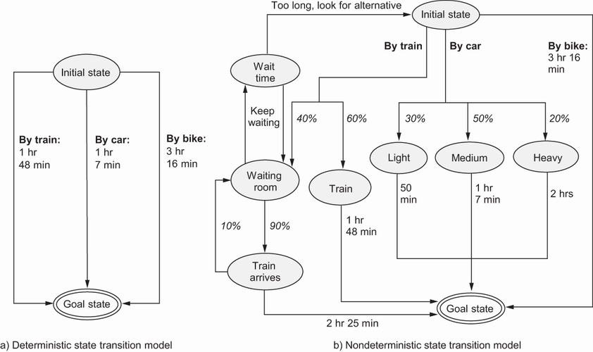
The commute diagram contrasts a deterministic route estimate with multiple possible outcomes after an action. section 12.1.1




