The Traveling Salesman Problem (TSP) asks for a tour through specified locations that visits each one exactly once and returns to the starting point. Model locations as graph vertices, connections as weighted edges, and the tour cost as the sum of distances between adjacent vertices. section 17.2
TSP is an NP-complete problem: candidate tours can be checked in polynomial time, but no known deterministic algorithm solves every instance in polynomial time. Exhaustive search quickly becomes impractical, with 10 cities producing about 3.6 million sequences, 15 producing about 1.3 trillion, and 20 producing about 2.4 × 10^18. section 17.2
A practical TSP workflow separates representation, evaluation, and search:
- Encode each candidate as a permutation of the graph’s vertices, with every vertex appearing once. section 18.2.1
- Evaluate a candidate by summing the distances between adjacent vertices; minimize this cost. section 18.2.1
- Use simulated annealing or genetic algorithms when exhaustive enumeration grows too large. section 17.0 section 18.2.1
A small permutation space
For six cities, there are 720 possible vertex permutations, making it feasible to display the complete cost landscape or brute-force the minimum. A larger map with 10 cities already takes several minutes to enumerate all 3.6 million permutations. section 17.2.2
Figure 17.8 An example map, mixing the DC Universe’s cities and other real ones, with some distances: because this is a complete graph with close to fifty edges, we are only showing a few numbers, almost only for the edges in the best tour (the thicker edges).
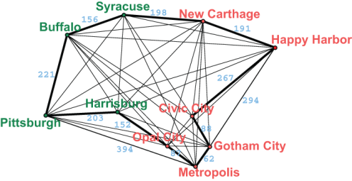
Use the map to inspect a weighted city graph and the highlighted edges forming a low-cost tour. section 17.2
TSP reasoning applies to delivery, school-bus routing, mail services, farming, service-call scheduling, printed-circuit-board drilling and soldering, and genome sequencing. Exact optimization trades rapidly increasing computation for certainty; approximation trades certainty for workable planning. section 17.2.6 section 17.2





