Upsampling expands a feature map back toward higher spatial resolution by generating values at additional locations. It commonly reverses earlier downsampling so outputs can align with the original image. section 11.3.2 section 17.2.2
Pixel-level image segmentation
A segmentation model first compresses a 200 × 200 image to a 25 × 25 × 256 feature map. Conv2DTranspose layers then expand it back to 200 × 200, allowing the final Conv2D layer to predict one class for every pixel. A stride-2 convolution that changes 100 × 100 × 64 to 50 × 50 × 128 can be followed by a stride-2 transposed convolution returning to 100 × 100 × 64. section 11.3.2
Common architectural choices include:
- Use Conv2DTranspose as a learned upsampling operation paired with earlier convolutional downsampling. section 11.3.2
- In a U-Net, match each upsampling block to a downsampling block and concatenate skip connections to preserve image detail. section 17.2.2
- Increase layer widths while downsampling and reduce them while upsampling. section 17.2.2
get_model <- function(img_size, num_classes) {

  conv <- function(..., padding = "same", activation = "relu")  #1
    layer_conv_2d(..., padding = padding, activation = activation)

  conv_transpose <- function(..., padding = "same", activation = "relu")
    layer_conv_2d_transpose(..., padding = padding, activation = activation)

  input <- keras_input(shape = c(img_size, 3))
  output <- input |>
    layer_rescaling(scale = 1/255) |>  #2
    conv(64, 3, strides = 2) |>
    conv(64, 3) |>
    conv(128, 3, strides = 2) |>
    conv(128, 3) |>
    conv(256, 3, strides = 2) |>
    conv(256, 3) |>
    conv_transpose(256, 3) |>
    conv_transpose(256, 3, strides = 2) |>
    conv_transpose(128, 3) |>
    conv_transpose(128, 3, strides = 2) |>
    conv_transpose(64, 3) |>
    conv_transpose(64, 3, strides = 2) |>
    conv(num_classes, 3, activation = "softmax")  #3

  keras_model(input, output)
}

model <- get_model(img_size = img_size, num_classes = 3)
model

Model: "functional"

┌─────────────────────────────────┬────────────────────────┬───────────────┐

│ Layer (type)                    │ Output Shape           │       Param # │

├─────────────────────────────────┼────────────────────────┼───────────────┤

│ input_layer (InputLayer)        │ (None, 200, 200, 3)    │             0 │

├─────────────────────────────────┼────────────────────────┼───────────────┤

│ rescaling (Rescaling)           │ (None, 200, 200, 3)    │             0 │

├─────────────────────────────────┼────────────────────────┼───────────────┤

│ conv2d (Conv2D)                 │ (None, 100, 100, 64)   │         1,792 │

├─────────────────────────────────┼────────────────────────┼───────────────┤

│ conv2d_1 (Conv2D)               │ (None, 100, 100, 64)   │        36,928 │

├─────────────────────────────────┼────────────────────────┼───────────────┤

│ conv2d_2 (Conv2D)               │ (None, 50, 50, 128)    │        73,856 │

├─────────────────────────────────┼────────────────────────┼───────────────┤

│ conv2d_3 (Conv2D)               │ (None, 50, 50, 128)    │       147,584 │

├─────────────────────────────────┼────────────────────────┼───────────────┤

│ conv2d_4 (Conv2D)               │ (None, 25, 25, 256)    │       295,168 │

├─────────────────────────────────┼────────────────────────┼───────────────┤

│ conv2d_5 (Conv2D)               │ (None, 25, 25, 256)    │       590,080 │

└─────────────────────────────────┴────────────────────────┴───────────────┘

┌─────────────────────────────────┬────────────────────────┬───────────────┐

│ conv2d_transpose                │ (None, 25, 25, 256)    │       590,080 │

│ (Conv2DTranspose)               │                        │               │

├─────────────────────────────────┼────────────────────────┼───────────────┤

│ conv2d_transpose_1              │ (None, 50, 50, 256)    │       590,080 │

│ (Conv2DTranspose)               │                        │               │

├─────────────────────────────────┼────────────────────────┼───────────────┤

│ conv2d_transpose_2              │ (None, 50, 50, 128)    │       295,040 │

│ (Conv2DTranspose)               │                        │               │

├─────────────────────────────────┼────────────────────────┼───────────────┤

│ conv2d_transpose_3              │ (None, 100, 100, 128)  │       147,584 │

│ (Conv2DTranspose)               │                        │               │

├─────────────────────────────────┼────────────────────────┼───────────────┤

│ conv2d_transpose_4              │ (None, 100, 100, 64)   │        73,792 │

│ (Conv2DTranspose)               │                        │               │

├─────────────────────────────────┼────────────────────────┼───────────────┤

│ conv2d_transpose_5              │ (None, 200, 200, 64)   │        36,928 │

│ (Conv2DTranspose)               │                        │               │

├─────────────────────────────────┼────────────────────────┼───────────────┤

│ conv2d_6 (Conv2D)               │ (None, 200, 200, 3)    │         1,731 │

└─────────────────────────────────┴────────────────────────┴───────────────┘

 Total params: 2,880,643 (10.99 MB)

 Trainable params: 2,880,643 (10.99 MB)

 Non-trainable params: 0 (0.00 B)
The complete R/Keras segmentation model shows a convolutional encoder followed by Conv2DTranspose layers that restore spatial resolution. section 11.3.2
Figure 17.9 Our U-Net style denoising autoencoder architecture
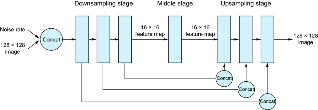
The U-Net diagram makes the mirrored downsampling and upsampling stages, plus their detail-preserving connections, easier to follow. section 17.2.2



