Weight decay is L2 regularization: it adds a penalty based on the sum of squared model weights, encouraging smaller, more evenly distributed coefficients without generally making them zero. This can reduce overfitting and stabilize models when features are correlated, such as molecular fingerprints. section 3.4.1
Use weight decay by considering three practical points:
- Tune the regularization parameter λ: larger values impose stronger constraints and produce simpler models. section 3.4.1
- Balance underfitting and overfitting: excessive regularization raises training error, while insufficient regularization can produce high-variance models that generalize poorly. section 4.4.3
- Compare training and validation performance across regularization values instead of treating a single model score as sufficient evidence. section 4.4.3
Molecular generation with VAE-CYC
A VAE-CYC molecular generator uses a conservative learning rate of 0.0001 with weight decay regularization, alongside dropout, word dropout, and free bits. Here, weight decay is one component of a broader strategy for producing useful molecular representations and generation behavior. section 10.4.5
Figure 3.16 Our model weights are exceedingly high given the model’s output space.
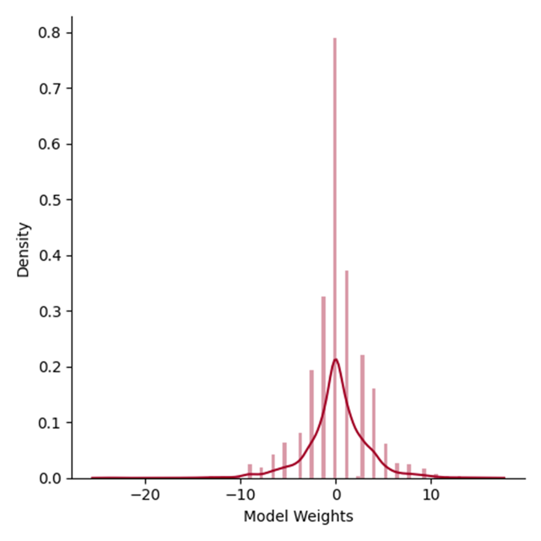
Inspect the weight-magnitude visualization to connect the regularization penalty with unusually large model weights. section 3.4.1
Figure 4.20 Validation curves for SVR and preprocessing hyperparameters.
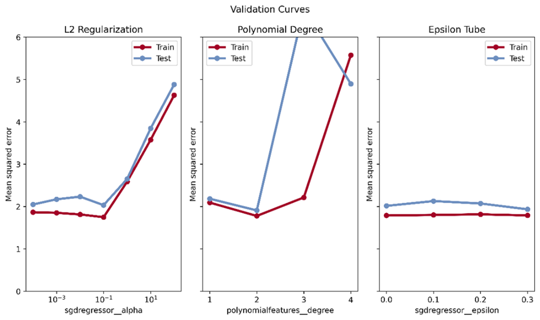
Use the validation curves to examine how L2 regularization changes SVR complexity and the gap between training and test performance. section 4.4.3