3 Introducing Dask DataFrames

In the previous chapter, we started exploring how Dask uses DAGs to coordinate and manage complex tasks across many machines. However, we only looked at some simple examples using the Delayed API to help illustrate how Dask code relates to elements of a DAG. In this chapter, we’ll begin to take a closer look at the DataFrame API. We’ll also start working through the NYC Parking Ticket data following a fairly typical data science workflow. This workflow and their corresponding chapters can be seen in figure 3.1.

Dask DataFrames wrap Delayed objects around Pandas DataFrames to allow you to operate on more sophisticated data structures. Rather than writing your own complex web of functions, the DataFrame API contains a whole host of complex transformation methods such as Cartesian products, joins, grouping operations, and so on, that are useful for common data manipulation tasks. Before we cover those operations in depth, which we will do in chapter 5, we’ll start our exploration of Dask by addressing some necessary background knowledge for data gathering. More specifically, we’ll look at how Dask DataFrames are well suited to manipulate structured data, which is data that consists of rows and columns. We’ll also look at how Dask can support parallel processing and handle large datasets by chunking data into smaller pieces called partitions. Plus, we’ll look at some performance-maximizing best practices throughout the chapter.

3.1 Why use DataFrames?

The shape of data found “in the wild” is usually described one of two ways: structured or unstructured. Structured data is made up of rows and columns: from the humble spreadsheet to complex relational database systems, structured data is an intuitive way to store information. Figure 3.2 shows an example of a structured dataset with rows and columns.

It’s natural to gravitate toward this format when thinking about data because the structure helps keep related bits of information together in the same visual space. A row represents a logical entity: in the spreadsheet, each row represents a person. Rows are made up of one or more columns, which represent things we know about each entity. In the spreadsheet, we’ve captured each person’s last name, first name, date of birth, and a unique identifier. Many kinds of data can be fit into this shape: transactional data from point-of-sale systems, results from a marketing survey, clickstream data, and even image data once it’s been specially encoded.

Because of the way that structured data is organized and stored, it’s easy to think of many different ways to manipulate the data. For example, we could find the earliest date of birth in the dataset, filter people out that don’t match a certain pattern, group people together by their last name, or sort people by their first name. Compare that with how the data might look if we stored it in several list objects.

In listing 3.1, the columns are stored as separate lists. Although it’s still possible to do all the transformations previously suggested, it’s not immediately evident that the four lists are related to each other and form a complete dataset. Furthermore, the code required for operations like grouping and sorting on this data would be quite complex and require a substantial understanding of data structures and algorithms to write code that performs efficiently. Python offers many different data structures that we could use to represent this data, but none are as intuitive for storing structured data as the DataFrame.

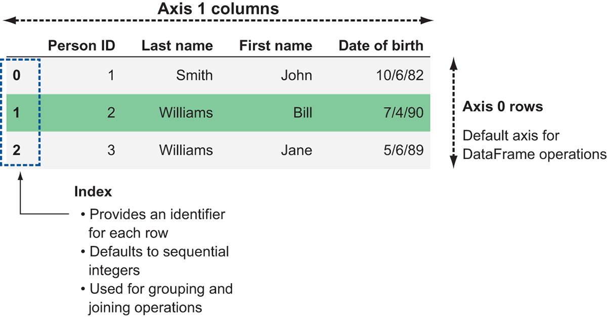
Like a spreadsheet or a database table, DataFrames are organized into rows and columns. However, we have a few additional terms to be aware of when working with DataFrames: indexes and axes. Figure 3.3 displays the anatomy of a DataFrame.

The example in figure 3.3 shows a DataFrame representation of the structured data from figure 3.2. Notice the additional labels on the diagram: rows are referred to as “axis 0” and columns are referred to as “axis 1.” This is important to remember when working with DataFrame operations that reshape the data. DataFrame operations default to working along axis 0, so unless you explicitly specify otherwise, Dask will perform operations row-wise.

The other area highlighted in figure 3.3 is the index. The index provides an identifier for each row. Ideally, these identifiers should be unique, especially if you plan to use the index as a key to join with another DataFrame. However, Dask does not enforce uniqueness, so you can have duplicate indices if necessary. By default, DataFrames are created with a sequential integer index like the one seen in figure 3.3. If you want to specify your own index, you can set one of the columns in the DataFrame to be used as an index, or you can derive your own Index object and assign it to be the index of the DataFrame. We cover common indexing functions in-depth in chapter 5, but the importance of indices in Dask cannot be overstated: they hold the key to distributing DataFrame workloads across clusters of machines. With that in mind, we’ll now take a look at how indices are used to form partitions.

3.2 Dask and Pandas

As mentioned a few times, Pandas is a very popular and powerful framework for analyzing structured data, but its biggest limitation is that it was not designed with scalability in mind. Pandas is exceptionally well suited for handling small structured datasets and is highly optimized to perform fast and efficient operations on data stored in memory. However, as we saw in our hypothetical kitchen scenario in chapter 1, as the volume of work increases substantially it can be a better choice to hire additional help and spread the tasks across many workers. This is where Dask’s DataFrame API comes in: by providing a wrapper around Pandas that intelligently splits huge data frames into smaller pieces and spreads them across a cluster of workers, operations on huge datasets can be completed much more quickly and robustly.

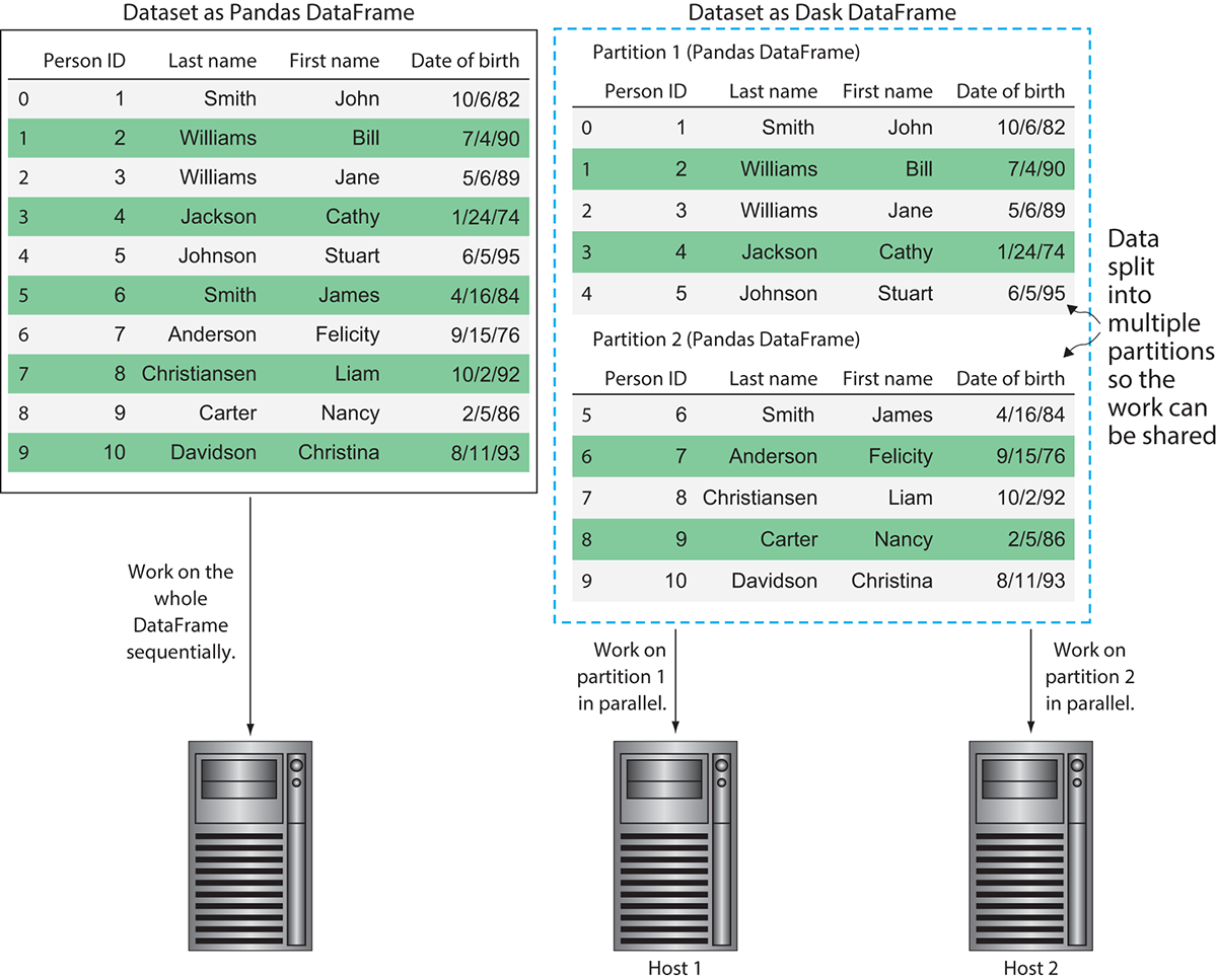
The different pieces of the DataFrame that Dask oversees are called partitions. Each partition is a relatively small DataFrame that can be dispatched to any worker and maintains its full lineage in case it must be reproduced. Figure 3.4 demonstrates how Dask uses partitioning for parallel processing.

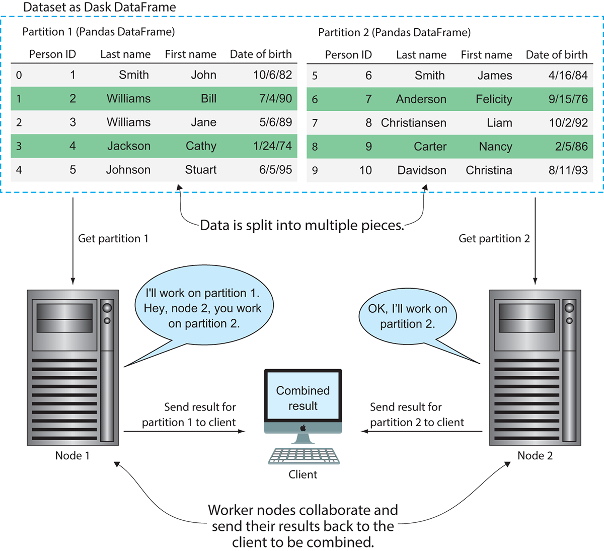
In figure 3.4, you can see the difference between how Pandas would handle the dataset and how Dask would handle the dataset. Using Pandas, the dataset would be loaded into memory and worked on sequentially one row at a time. Dask, on the other hand, can split the data into multiple partitions, allowing the workload to be parallelized. This means if we had a long-running function to apply over the DataFrame, Dask could complete the work more efficiently by spreading the work out over multiple machines. However, it should be noted that the DataFrame in figure 3.4 is used only for the sake of example. As mentioned previously, the task scheduler does introduce some overhead into the process, so using Dask to process a DataFrame with only 10 rows would likely not be the fastest solution. Figure 3.5 shows an example of how two hosts might coordinate work on this partitioned dataset in more detail.

As node 1 is driving the computation and telling node 2 what to do, it is currently taking on the role of the task scheduler. Node 1 tells node 2 to work on partition 2 while node 1 works on partition 1. Each node finishes its processing tasks and send its part of the result back to the client. The client then assembles the pieces of the results and displays the output.

3.2.1 Managing DataFrame partitioning

Since partitioning can have such a significant impact on performance, you might be worried that managing partitioning will be a difficult and tedious part of constructing Dask workloads. However, fear not: Dask tries to help you get as much performance as possible without manual tuning by including some sensible defaults and heuristics for creating and managing partitions. For example, when reading in data using the read_csv method of Dask DataFrames, the default partition size is 64 MB each (this is also known as the default blocksize). While 64 MB might seem quite small given that modern servers tend to have tens of gigabytes of RAM, it is an amount of data that is small enough that it can be quickly transported over the network if necessary, but large enough to minimize the likelihood that a machine will run out of things to do while waiting for the next partition to arrive. Using either the default or a user-specified blocksize, the data will be split into as many partitions as necessary so that each partition is no larger than the blocksize. If you desire to create a DataFrame with a specific number of partitions instead, you can specify that when creating the DataFrame by passing in the npartitions argument.

In listing 3.2, we created a Dask DataFrame and explicitly split it into two partitions using the npartitions argument. Normally, Dask would have put this dataset into a single partition because it is quite small.

Listing 3.3 shows a couple useful attributes of Dask DataFrames that can be used to inspect how a DataFrame is partitioned. The first attribute, divisions, (0, 5, 9), shows the boundaries of the partitioning scheme (remember that partitions are created on the index). This might look strange since there are two partitions but three boundaries. Each partition’s boundary consists of pairs of numbers from the list of divisions. The boundary for the first partition is “from 0 up to (but not including) 5,” meaning it will contain rows 0, 1, 2, 3, and 4. The boundary for the second partition is “from 5 through (and including) 9,” meaning it will contain rows 5, 6, 7, 8, and 9. The last partition always includes the upper boundary, whereas the other partitions go up to but don’t include their upper boundary.

The second attribute, npartitions, simply returns the number of partitions that exist in the DataFrame.

Listing 3.4 shows how to use the map_partitions method to count the number of rows in each partition. map_partitions generally applies a given function to each partition. This means that the result of the map_partitions call will return a Series equal in size to the number of partitions the DataFrame currently has. Since we have two partitions in this DataFrame, we get two items back in the result of the call. The output shows that each partition contains five rows, meaning Dask split the DataFrame into two equal pieces.

Sometimes it may be necessary to change the number of partitions in a Dask DataFrame. Particularly when your computations include a substantial amount of filtering, the size of each partition can become imbalanced, which can have negative performance consequences on subsequent computations. The reason for this is because if one partition suddenly contains a majority of the data, all the advantages of parallelism are effectively lost. Let’s look at an example of this. First, we’ll derive a new DataFrame by applying a filter to our original DataFrame that removes all people with the last name Williams. We’ll then inspect the makeup of the new DataFrame by using the same map_partitions call to count the rows per partition.

Notice what happened: the first partition now only contains three rows, and the second partition has the original five. People with the last name of Williams happened to be in the first partition, so our new DataFrame has become rather unbalanced.

The second two lines of code in the listing aim to fix the imbalance by using the repartition method on the filtered DataFrame. The npartitions argument here works the same way as the npartitions argument used earlier when we created the initial DataFrame. Simply specify the number of partitions you want and Dask will figure out what needs to be done to make it so. If you specify a lower number than the current number of partitions, Dask will combine existing partitions by concatenation. If you specify a higher number than the current number of partitions, Dask will split existing partitions into smaller pieces. You can call repartition at any time in your program to initiate this process. However, like all other Dask operations, it’s a lazy computation. No data will actually get moved around until you make a call such as compute, head, and so on. Calling the map_partitions function again on the new DataFrame, we can see that the number of partitions has been reduced to one, and it contains all eight of the rows. Note that if you repartition again, this time increasing the number or partitions, the old divisions (0, 5, 9) will be retained. If you want to split the partitions evenly, you will need to manually update the divisions to match your data.

3.2.2 What is the shuffle?

Now that we’ve learned that partitioning is important, explored how Dask handles partitioning, and learned what you can do to influence it, we’ll round out this discussion by learning about a frequent challenge that arises in distributed computing: dealing with the shuffle. No, I’m not talking about the dance move—frankly, I wouldn’t be the best source of dance advice! In distributed computing, the shuffle is the process of broadcasting all partitions to all workers. Shuffling the data is necessary when performing sorting, grouping, and indexing operations, because each row needs to be compared to every other row in the entire DataFrame to determine its correct relative position. This is a time-expensive operation, because it necessitates transferring large amounts of data over the network. Let’s see what this might look like.

In figure 3.6, we’re seeing what would happen with our DataFrame if we want to group our data by Last Name. For example, we might want to find the eldest person by last name. For the majority of the data, it’s no problem. Most of the last names in this dataset are unique. As you can see in the data in figure 3.6, there are only two cases in which we have multiple people with the same last name: Williams and Smith. For the two people named Williams, they are in the same partition, so server 1 has all the information it needs locally to determine that the oldest Williams was born in 1989. However, for the people named Smith, there’s one Smith in partition 1 and one Smith in partition 2. Either server 1 will have to send its Smith to server 2 to make the comparison, or server 2 will have to send server 1 its Smith. In both cases, for Dask to be able to compare the birthdates of each Smith, one of them will have to be shipped over the network.

Depending on what needs to be done with the data, completely avoiding shuffle operations might not be feasible. However, you can do a few things to minimize the need for shuffling the data. First, ensuring that the data is stored in a presorted order will eliminate the need to sort the data with Dask. If possible, sorting the data in a source system, such as a relational database, can be faster and more efficient than sorting the data in a distributed system. Second, using a sorted column as the DataFrame’s index will enable greater efficiency with joins. When the data is presorted, lookup operations are very fast because the partition where a certain row is kept can be easily determined by using the divisions defined on the DataFrame. Finally, if you must use an operation that triggers a shuffle, persist the result if you have the resources to do so. This will prevent having to repeat shuffling the data again if the DataFrame needs to be recomputed.

3.3 Limitations of Dask DataFrames

Now that you have a good idea of what the DataFrame API is useful for, it will be helpful to close the chapter by covering a few limitations that the DataFrame API has.

First and foremost, Dask DataFrames do not expose the entire Pandas API. Even though Dask DataFrames are made up of smaller Pandas DataFrames, some functions that Pandas does well are simply not conducive to a distributed environment. For example, functions that would alter the structure of the DataFrame, such as insert and pop, are not supported because Dask DataFrames are immutable. Some of the more complex window operations are also not supported, such as expanding and EWM methods, as well as complex transposition methods like stack/unstack and melt, because of their tendency to cause a lot of data shuffling. Oftentimes, these expensive operations don’t really need to be performed on the full, raw dataset. In those cases, you should use Dask to do all your normal data prep, filtering, and transformation, then dump the final dataset into Pandas. You will then be able to perform the expensive operations on the reduced dataset. Dask’s DataFrame API makes it very easy to interoperate with Pandas DataFrames, so this pattern can be very useful when analyzing data using Dask DataFrames.

The second limitation is with relational-type operations, such as join/merge, groupby, and rolling. Although these operations are supported, they are likely to involve a lot of shuffling, making them performance bottlenecks. This can be minimized, again, either by using Dask to prepare a smaller dataset that can be dumped into Pandas, or by limiting these operations to only use the index. For example, if we wanted to join a DataFrame of people to a DataFrame of transactions, that computation would be significantly faster if both datasets were sorted and indexed by the Person ID. This would minimize the likelihood that each person’s records are spread out across many partitions, in turn making shuffles more efficient.

Third, indexing has a few challenges due to the distributed nature of Dask. If you wish to use a column in a DataFrame as an index in lieu of the default numeric index, it will need to be sorted. If the data is stored presorted, this becomes no problem at all. If the data is not presorted, it can be very slow to sort the entire DataFrame because it requires a lot of shuffling. Effectively, each partition first needs to be sorted, then needs to be merged and sorted again with every other partition. Sometimes it may be necessary to do this, but if you can proactively store your data presorted for the computations you need, it will save you a lot of time.

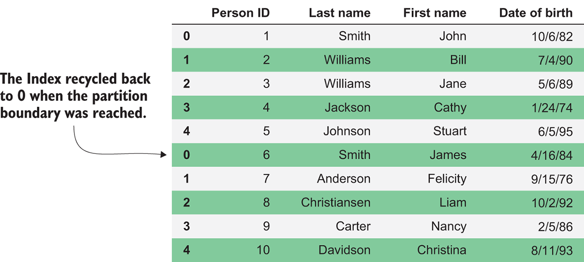
The other significant difference you may notice with indexing is how Dask handles the reset_index method. Unlike Pandas, where this will recalculate a new sequential index across the entire DataFrame, the method in Dask DataFrames behaves like a map_partitions call. This means that each partition will be given its own sequential index that starts at 0, so the whole DataFrame will no longer have a unique sequential index. In figure 3.7, you can see the effect of this.

Each partition contained five rows, so once we called reset_index, the index of the first five rows remains the same, but the next five rows, which are contained in the next partition, start over at 0. Unfortunately, there’s no easy way to reset the index in a partition-aware way. Therefore, use the reset_index method carefully and only if you don’t plan to use the resulting sequential index to join, group, or sort the DataFrame.

Finally, since a Dask DataFrame is made up of many Pandas DataFrames, operations that are inefficient in Pandas will also be inefficient in Dask. For example, iterating over rows by using the apply and iterrows methods is notoriously inefficient in Pandas. Therefore, following Pandas best practices will give you the best performance possible when using Dask DataFrames. If you’re not well on your way to mastering Pandas yet, continuing to sharpen your skills will not only benefit you as you get more familiar with Dask and distributed workloads, but it will help you in general as a data scientist!

Summary