9 Working with Bags and Arrays

The majority of this book focuses on using DataFrames for analyzing structured data, but our exploration of Dask would not be complete without mentioning the two other high-level Dask APIs: Bags and Arrays. When your data doesn’t fit neatly in a tabular model, Bags and Arrays offer additional flexibility. DataFrames are limited to only two dimensions (rows and columns), but Arrays can have many more. The Array API also offers additional functionality for certain linear algebra, advanced mathematics, and statistics operations. However, much of what’s been covered already through working with DataFrames also applies to working with Arrays—just as Pandas and NumPy have many similarities. In fact, you might recall from chapter 1 that Dask DataFrames are parallelized Pandas DataFrames and Dask Arrays are parallelized NumPy arrays.

Bags, on the other hand, are unlike any of the other Dask data structures. Bags are very powerful and flexible because they are parallelized general collections, most like Python’s built-in List object. Unlike Arrays and DataFrames, which have predetermined shapes and datatypes, Bags can hold any Python objects, whether they are custom classes or built-in types. This makes it possible to contain very complicated data structures, like raw text or nested JSON data, and navigate them with ease.

Working with unstructured data is becoming more commonplace for data scientists, especially data scientists who are working independently or in small teams without a dedicated data engineer. Take the following, for example.

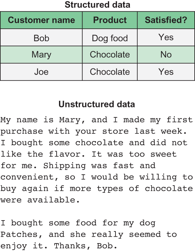
In figure 9.1, the same data is presented two different ways: the upper half shows some examples of product reviews as structured data with rows and columns, and the lower half shows the raw review text as unstructured data. If the only information we care about is the customer’s name, the product they purchased, and whether or not they were satisfied, the structured data gives us this information at a glance without any ambiguity. Every value in the Customer Name column is always the customer’s name. Conversely, the varying length, writing style, and free-form nature of the raw text makes it unclear what data is relevant for analysis and requires some sort of parsing and interpretation to extract the relevant data. In the first review, the reviewer’s name (Mary) is the fourth word of the review. However, the second reviewer put his name (Bob) at the very end of his review. These inconsistencies make it difficult to use a rigid data structure like a DataFrame or an Array to organize the information. Instead, the flexibility of Bags really shines here: whereas a DataFrame or Array always has a fixed number of columns, a Bag can contain strings, lists, or any other element of varying length.

In fact, the typical use case that involves working with unstructured data comes from analyzing text data scraped from web APIs, such as product reviews, tweets from Twitter, or ratings from services like Yelp and Google Reviews. Therefore, we’ll walk through an example of using Bags to parse and prepare unstructured text data; then we’ll look at how to map and derive structured data from Bags to Arrays.

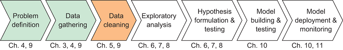
Figure 9.2 is our familiar workflow diagram, but it might be a bit surprising because we’ve stepped back to the first three tasks! Since we’re starting with a new problem and dataset, rather than progressing onward from chapter 8, we’ll be revisiting the first three elements of our workflow, this time with the focus on unstructured data. Many of the concepts that were covered in chapters 4 and 5 are the same, but we will look at how to technically achieve the same results when the data doesn’t come in a tabular format such as CSV.

As a motivating example for this chapter, we’ll look at a set of product reviews from Amazon.com sourced by Stanford University’s Network Analysis Project. You can download the data from here: https://goo.gl/yDQgfH. To learn more about how the dataset was created, see McAuley and Leskovec’s paper “From Amateurs to Connoisseurs: Modeling the Evolution of User Expertise through Online Reviews” (Stanford, 2013).

9.1 Reading and parsing unstructured data with Bags

After you’ve downloaded the data, the first thing you need to do is properly read and parse the data so you can easily manipulate it. The first scenario we’ll walk through is

Using the Amazon Fine Foods Revie ws dataset, determine its format and parse the data into a Bag of dictionaries.

This particular dataset is a plain text file. You can open it with any text editor and start to make sense of the layout of the file. The Bag API offers a few convenience methods for reading text files. In addition to plain text, the Bag API is also equipped to read files in the Apache Avro format, which is a popular binary format for JSON data and is usually denoted by a file ending in .avro. The function used to read plain text files is read_text, and has only a few parameters. In its simplest form, all it needs is a filename. If you want to read multiple files into one Bag, you can alternatively pass a list of filenames or a string with a wildcard (such as *.txt). In this instance, all the files in the list of filenames should have the same kind of information; for example, log data collected over time where one file represents a single day of logged events. The read_text function also natively supports most compression schemes (such as GZip and BZip), so you can leave the data compressed on disk. Leaving your data compressed can, in some cases, offer significant performance gains by reducing the load on your machine’s input/output subsystem, so it’s generally a good idea. Let’s take a look at what the read_text function will produce.

As you’ve probably come to expect by now, the read_text operation produces a lazy object that won’t get evaluated until we actually perform a compute-type operation on it. The Bag’s metadata indicates that it will read the entire data in as one partition. Since the size of this file is rather small, that’s probably OK. However, if we wanted to manually increase parallelism, read_text also takes an optional blocksize parameter that allows you to specify how large each partition should be in bytes. For instance, to split the roughly 400 MB file into four partitions, we could specify a blocksize of 100,000,000 bytes, which equates to 100 MB. This will cause Dask to divide the file into four partitions.

9.1.1 Selecting and viewing data from a Bag

Now that we’ve created a Bag from the data, let’s see how the data looks. The take method allows us to look at a small subset of the items in the Bag, just as the head method allows us to do the same with DataFrames. Simply specify the number of items you want to view, and Dask prints the result.

As you can see from the result of listing 9.2, each element of the Bag currently represents a line in the file. However, this structure will prove to be problematic for our analysis. There is an obvious relationship between some of the elements. For example, the review/score element being displayed is the review score for the product ID preceding it (B001E4KFG0). But since there is nothing structurally relating these elements, it would be difficult to do something like calculate the mean review score for item B001E4KFG0. Therefore, we should add a bit of structure to this data by grouping the elements that are associated together into a single object.

9.1.2 Common parsing issues and how to overcome them

A common issue that arises when working with text data is making sure the data is being read using the same character encoding as it was written in. Character encoding is used to map raw data stored as binary into symbols that we humans can identify as letters. For example, the capital letter J is represented in binary as 01001010 using the UTF-8 encoding. If you open a text file in a text editor using UTF-8 to decode the file, everywhere 01001010 is encountered in the file, it will be translated to a J before it is displayed on the screen.

Using the correct character encoding makes sure the data will be read correctly and you won’t see any garbled text. By default, the read_text function assumes that the data is encoded using UTF-8. Since Bags are inherently lazy, the validity of this assumption isn’t checked ahead of time, meaning you’ll be tipped off that there’s a problem only when you perform a function over the entire dataset. For example, if we want to count the number of items in the Bag, we could use the count function.

The count function, which looks exactly like the count function from the DataFrame API, fails with a UnicodeDecodeError exception. This tells us that the file is probably not encoded in UTF-8 since it can’t be parsed. These issues typically arise if the text uses any kind of characters that aren’t used in the English alphabet (such as accent marks, Hanzi, Hiragana, and Abjads). If you are able to ask the producer of the file which encoding was used, you can simply add the encoding to the read_text function using the encoding parameter. If you’re not able to find out the encoding that the file was saved in, a bit of trial and error is necessary to determine which encoding to use. A good place to start is trying the cp1252 encoding, which is the standard encoding used by Windows. In fact, this example dataset was encoded using cp1252, so we can modify the read_text function to use cp1252 and try our count operation again.

This time, the file is able to be parsed completely and we’re shown that the file contains 5.11 million lines.

9.1.3 Working with delimiters

With the encoding problem solved, let’s look at how we can add the structure we need to group the attributes of each review together. Since the file we’re working with is just one long string of text data, we can look for patterns in the text that might be useful for dividing the text into logical chunks. Figure 9.3 shows a few hints as to where some useful patterns in the text are.

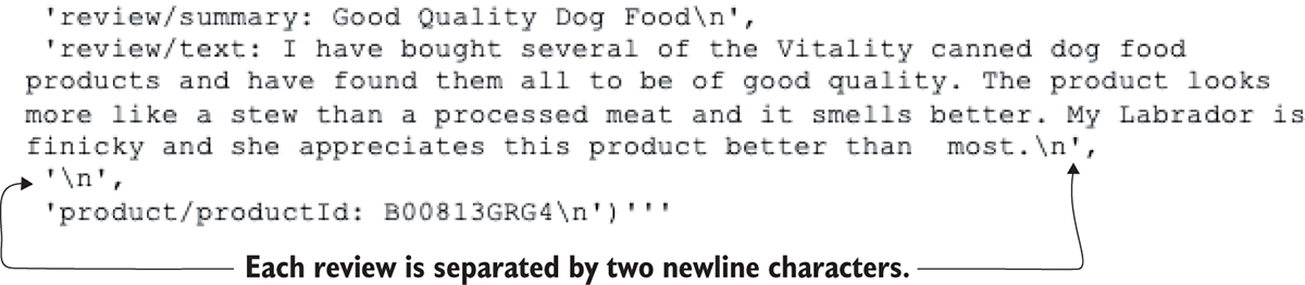
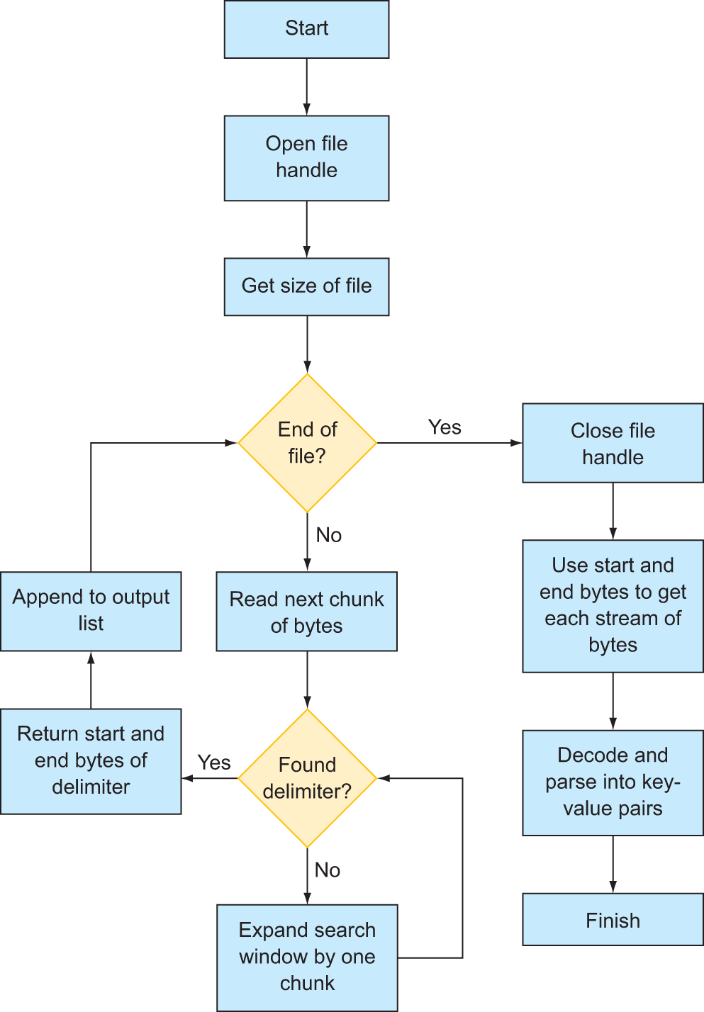
In this particular example, the author of the dataset has put two newline characters (which show up as \n) between each review. We can use this pattern as a delimiter to split the text into chunks, where each chunk of text contains all attributes of the review, such as the product ID, the rating, the review text, and so on. We will need to manually parse the text file using some functions from the Python standard library. What we want to avoid doing, however, is reading the entire file into memory in order to do this. Although this file could comfortably fit into memory, an example that reads the entire file into memory would not work once you start working with datasets that exceed the limits of your machine (and it would defeat the whole purpose of parallelism to boot!). Therefore, we will use Python’s file iterator to stream the file a small chunk at a time, search the text in the buffer for our desired delimiter, mark the position in the file where a review starts and ends, and then advance the buffer to find the position of the next review. We’ll end up with a list of Delayed objects that have pointers to the start and end of each review, which can further be parsed into a dictionary of key-value pairs. The full process from start to finish is outlined in the flowchart in figure 9.4.

First, we’ll define a function that searches a part of a file for our specified delimiter. With Python’s file handle system, it’s possible to stream data in from a file starting at a specific byte number and stopping at a specific byte number. For instance, the beginning of the file is byte 0. The next character is byte 1, and so forth. Rather than load the whole file into memory, we can load chunks in at a time. For instance, we could load 1000 bytes of data starting at byte 5000. The space in memory we’re loading the 1000 bytes of data into is called a buffer. We can decode the buffer from raw bytes to a string object, and then use all the string manipulation functions available to us in Python, such as find, strip, split, and so on. And, since the buffer space is only 1000 bytes in this example, that’s approximately all the memory we will use.

We need a function that will

Here’s a function that will do that.

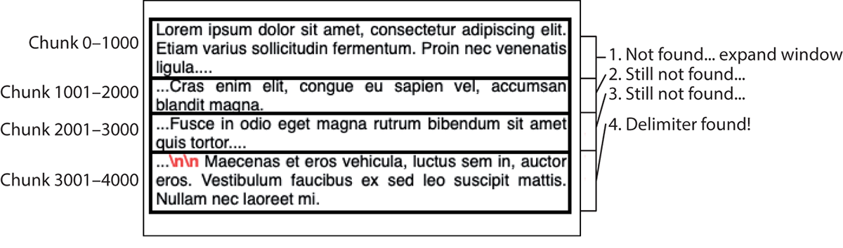
Given a file handle and a starting position, this function will find the next occurrence of the delimiter. The recursive function call that occurs if the delimiter isn’t found in the current buffer adds the current buffer size to the span_index parameter. This is how the window continues to expand if the delimiter search fails. The first time the function is called, the span_index will be 0. With a default blocksize of 1000, this means the function will read the next 1000 bytes after the starting position (1000 blocksize + 0 span_index). If the find fails, the function is called again after incrementing the span_index by 1000. Then it will then try again by searching the next 2000 bytes after the starting position (1000 blocksize + 1000 span_index). If the find continues to fail, the search window will keep expanding by 1000 bytes until a delimiter is finally found or the end of the file is reached. A visual example of this process can be seen in figure 9.5.

To find all instances of the delimiter in the file, we can call this function inside a loop that will iterate chunk by chunk until the end of the file is reached. To do this, we’ll use a while loop.

Essentially this code accomplishes four things:

After initializing a few variables, we enter the loop starting at byte 0. Every time a delimiter is found, the current position is advanced to just after the position of the delimiter. For instance, if the first delimiter starts at byte 627, the first review is made up of bytes 0 through 626. Bytes 0 and 626 would be appended to the output list, and the current position would be advanced to 628. We add two to the next_position variable because the delimiter is two bytes (each ‘\n’ is one byte). Therefore, since we don’t really care about keeping the delimiters as part of the final review objects, we’ll skip over them. The search for the next delimiter will pick up at byte 629, which should be the first character of the next review. This continues until the end of the file is reached. By then we have a list of tuples. The first element in each tuple represents the starting byte, and the second element in each tuple represents the number of bytes to read after the starting byte. The list of tuples looks like this:

Before moving on, check the length of the output list using the len function. The list should contain 568,454 elements.

Now that we have a list containing all the byte positions of the reviews, we need to create some instructions to transform the list of addresses into a list of actual reviews. To do that, we’ll need to create a function that takes a starting position and a number of bytes as input, reads the file at the specified byte location, and returns a parsed review object. Because there are thousands of reviews to be parsed, we can speed up this process using Dask. Figure 9.6 demonstrates how we can divide up the work across multiple workers.

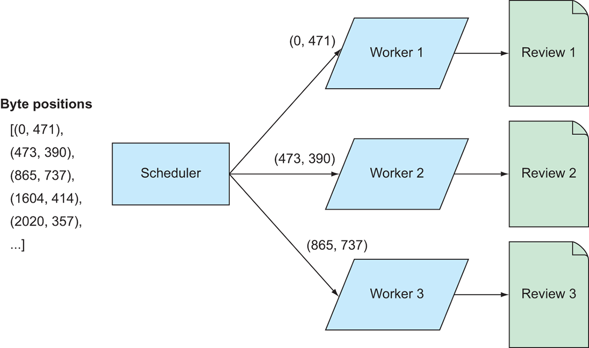
Effectively, the list of addresses will be divided up among the workers; each worker will open the file and parse the reviews at the byte positions it receives. Since the reviews are stored as JSON, we will create a dictionary object for each review to store its attributes. Each attribute of the review looks something like this: 'review/userId: A3SGXH7AUHU8GW\n', so we can exploit the pattern of each key ending in ': ' to split the data into key-value pairs for the dictionaries. The next listing shows a function that will do that.

Now that we have a function that will parse a specified part of the file, we need to actually send those instructions out to the workers so they can apply the parsing code to the data. We’ll now bring everything together and create a Bag that contains the parsed reviews.

The code in listing 9.8 does two things: first, we turn the list of byte addresses into a Bag using the from_sequence function of the Bag array. This creates a Bag that holds the same list of byte addresses as our original list, but now allows Dask to distribute the contents of the Bag to the workers. Next, the map function is called to transform each byte address tuple into its respective review object. Map effectively hands out the Bag of byte addresses and the instructions contained in the get_item function to the workers (remember that when Dask is running in local mode, the workers are independent threads on your machine). A new Bag called reviews is created, and when it is computed, it will output the parsed reviews. In listing 9.8, we pass in the get_item function inside of a lambda expression so we can keep the filename parameter fixed while dynamically inputting the start and end byte address from each item in the Bag. As before, this entire process is lazy. The result of listing 9.8 will show that a Bag has been created with 101 partitions. However, taking elements from the Bag will now result in a very different output!

Each element in the transformed Bag is now a dictionary that contains all attributes of the review! This will make analysis a lot easier for us. Additionally, if we count the items in the transformed Bag, we also get a far different result.

The number of elements in the Bag has been greatly reduced because we’ve assembled the raw text into logical reviews. This count also matches the number of reviews stated by Stanford on the dataset’s webpage, so we can be sure that we’ve correctly parsed the data without running into any more encoding issues! Now that our data is a bit easier to work with, we’ll look at some other ways we can manipulate data using Bags.

9.2 Transforming, filtering, and folding elements

Unlike lists and other generic collections in Python, Bags are not subscript-able, meaning it’s not possible to access a specific element of a Bag in a straightforward way. This can make data manipulation slightly more challenging until you become comfortable with thinking about data manipulation in terms of transformations. If you are familiar with functional programming or MapReduce style programming, this line of thinking comes naturally. However, it can seem a bit counterintuitive at first if you have a background of SQL, spreadsheets, and Pandas. If this is the case, don’t worry. With a bit of practice, you too will be able to start thinking of data manipulation in terms of transformations!

The next scenario we’ll use for motivation is the following:

Using the Amazon Fine Foods Reviews dataset, tag the review as being positive or negative by using the review score as a threshold.

9.2.1 Transforming elements with the map method

Let’s start easy—first, we’ll simply get all the review scores for the entire dataset. To do this, we’ll use the map function again. Rather than thinking about what we’re trying to do as getting the review scores, think about what we’re trying to do as transforming our Bag of reviews to a Bag of review scores. We need some kind of function that will take a review (dictionary) object in as an input and spit out the review score. A function that does that looks like this.

This is just plain old Python. We could pass any dictionary into this function, and if it contained a key of review/score, this function would cast the value to a float and return the value. If we map over our Bag of dictionaries using this function, it will transform each dictionary into a float containing the relevant review score. This is quite simple.

The review_scores Bag now contains all the raw review scores. The transformations you create can be any valid Python function. For instance, if we wanted to tag the reviews as being positive or negative based on the review score, we could use a function like this.

In listing 9.13, we mark a review as being positive if its score is greater than three stars; otherwise, we mark it as negative. You can see the new review/sentiment elements are displayed when we take some elements from the transformed Bag. However, be careful: while it may look like we’ve modified the original data since we’re assigning new key-value pairs to each dictionary, the original data actually remains the same. Bags, like DataFrames and Arrays, are immutable objects. What happens behind the scenes is each old dictionary being transformed to a copy of itself with the additional key-value pairs, leaving the original data intact. We can confirm this by looking at the original reviews Bag.

As you can see, the review/sentiment key is nowhere to be found. Just as when working with DataFrames, be aware of immutability to ensure you don’t run into any issues with disappearing data.

9.2.2 Filtering Bags with the filter method

The second important data manipulation operation with Bags is filtering. Although Bags don’t offer a way to easily access a specific element, say the 45th element in the Bag, they do offer an easy way to search for specific data. Filter expressions are Python functions that return True or False. The filter method maps the filter expression over the Bag, and any element that returns True when the filter expression is evaluated is retained. Conversely, any element that returns False when the filter expression is evaluated is discarded. For example, if we want to find all reviews of product B001E4KFG0, we can create a filter expression to return that data.

Listing 9.15 returns the data we requested, as well as a warning letting us know that there were fewer elements in the Bag than we asked for indicating there was only one review for the product we specified. We can also easily do fuzzy-matching searches. For example, we could find all reviews that mention “dog” in the review text.

And, just as with mapping operations, it’s possible to make filtering expressions more complex as well. To demonstrate, let’s use the following scenario for motivation:

Using the Amazon Fine Foods Reviews dataset, write a filter function that removes reviews that were not deemed “helpful” by other Amazon customers.

Amazon gives users the ability to rate reviews for their helpfulness. The review/helpfulness attribute represents the number of times a user said the review was helpful over the number of times users voted for the review. A helpfulness of 1/3 indicates that three users evaluated the review and only one found the review helpful (meaning the other two did not find the review helpful). Reviews that are unhelpful are likely to either be reviews where the reviewer unfairly gave a very low score or a very high score without justifying it in the review. It might be a good idea to eliminate unhelpful reviews from the dataset because they may not fairly represent the quality or value of a product. Let’s have a look at how unhelpful reviews are influencing the data by comparing the mean review score with and without unhelpful reviews. First, we’ll create a filter expression that will return True if more than 75% of users who voted found the review to be helpful, thereby removing any reviews below that threshold.

Unlike the simple filter expressions defined inline using lambda expressions in listings 9.15 and 9.16, we’ll define a function for this filter expression. Before we can evaluate the percentage of users that found the review helpful, we first have to calculate the percentage by parsing and transforming the raw helpfulness score. Again, we can do this in plain old Python using local scoped variables. We add some guards around the calculation to catch any potential divide-by-zero errors in the event no users voted on the review (note: practically, this means we assume reviews that haven’t been voted on are deemed unhelpful). If it’s had at least one vote, we return a Boolean expression that will evaluate to True if more than 75% of users found the review helpful. Now we can apply it to the data to see what happens.

9.2.3 Calculating descriptive statistics on Bags

As expected, all of the reviews in the filtered Bag are “helpful.” Now let’s take a look at how that affects the review scores.

In listing 9.19, we first extract the scores from the filtered Bag by mapping the get_score function over it. Then, we can call the mean method on each of the Bags that contain the review scores. After the means are computed, the output will display. Comparing the mean scores allows us to see if there’s any relationship between the helpfulness of reviews and the sentiment of the reviews. Are negative reviews typically seen as helpful? Unhelpful? Comparing the means allows us to answer this question. As can be seen, if we filter out the unhelpful reviews, the mean review score is actually a bit higher than the mean score for all reviews. This is most likely explained by the tendency of negative reviews to get downvoted if the reviewers don’t do a good job of justifying the negative score. We can confirm our suspicions by looking at the mean length of reviews that are helpful or unhelpful.

In listing 9.20, we’ve chained both map and filter operations together to produce our result. Since we already filtered out the helpful reviews, we can simply map the get_length function over the Bag of helpful reviews to extract the length of each review. However, we hadn’t isolated the unhelpful reviews before, so we did the following:

It looks like unhelpful reviews are indeed shorter than helpful reviews on average. This means that the longer a review is, the more likely it will be voted by the community to be helpful.

9.2.4 Creating aggregate functions using the foldby method

The last important data manipulation operation with Bags is folding. Folding is a special kind of reduce operation. While reduce operations have not been explicitly called out in this chapter, we’ve already seen a number of reduce operations throughout the book, as well as even in the previous code listing. Reduce operations, as you may guess by the name, reduce a collection of items in a Bag to a single value. For example, the mean method in the previous code listing reduces the Bag of raw review scores to a single value: the mean. Reduce operations typically involve some sort of aggregation over the Bag of values, such as summing, counting, and so on. Regardless of what the reduce operation does, it always results in a single value. Folding, on the other hand, allows us to add a grouping to the aggregation. A good example is counting the number of reviews by review score. Rather than count all the items in the Bag using a reduce operation, using a fold operation will allow us to count the number of items in each group. This means a fold operation reduces the number of elements in a Bag to the number of distinct groups that exist within the specified grouping. In the example of counting reviews by review score, this would result in reducing our original Bag down to five elements as there are five distinct review scores possible. Figure 9.7 shows an example of folding.

First, we need to define two functions to feed to the foldby method. These are called the binop and combine functions.

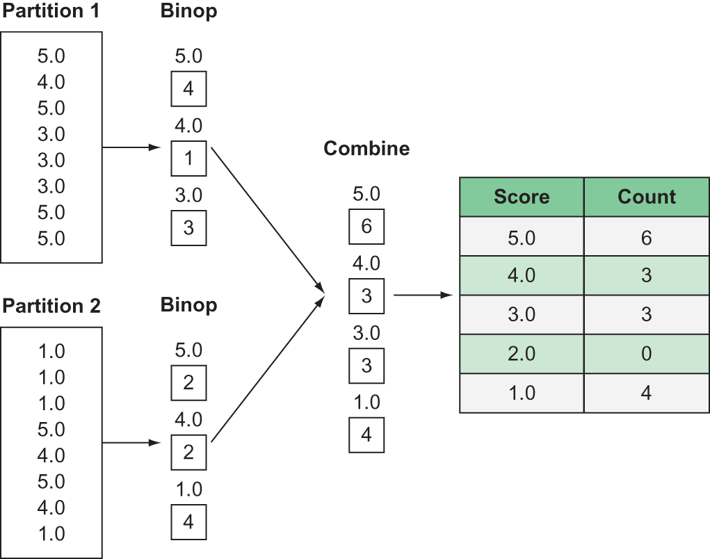
The binop function defines what should be done with the elements of each group, and always has two parameters: one for the accumulator and one for the element. The accumulator is used to hold the intermediate result across calls to the binop function. In this example, since our binop function is a counting function, it simply adds one to the accumulator each time the binop function is called. Since the binop function is called for every element in a group, this results in a count of items in each group. If the value of each element needs to be accessed, for instance if we wanted to sum the review scores, it can be accessed through the element parameter of the binop function. A sum function would simply add the element to the accumulator.

The combine function defines what should be done with the results of the binop function across the Bag’s partitions. For example, we might have reviews with a score of three in several partitions. We want to count the total number of three-star reviews across the entire Bag, so intermediate results from each partition should be summed together. Just like the binop function, the first argument of the combine function is an accumulator, and the second argument is an element. Constructing these two functions can be challenging, but you can effectively think of it as a “group by” operation. The binop function specifies what should be done to the grouped data, and the combine function defines what should be done with groups that exist across partitions.

Now let’s take a look at what this looks like in code.

The five required arguments of the foldby method, in order from left to right, are the key function, the binop function, an initial value for the binop accumulator, the combine function, and an initial value for the combine accumulator. The key function defines what the values should be grouped by. Generally, the key function will just return a value that’s used as a grouping key. In the previous example, it simply returns the value of the review score using the get_score function defined earlier in the chapter. The output of listing 9.21 looks like this.

What we’re left with after the code runs is a list of tuples, where the first element is the key and the second element is the result of the binop function. For example, there were 363,122 reviews that were given a five-star rating. Given the high mean review score, it shouldn’t come as any surprise that most of the reviews gave a five-star rating. It’s also interesting that there were more one-star reviews than there were two-star or three-star reviews. Nearly 75% of all reviews in this dataset were either five stars or one star—it seems most of our reviewers either absolutely loved their purchase or absolutely hated it. To get a better feel for the data, let’s dig a little bit deeper into the statistics of both the review scores and the helpfulness of reviews.

9.3 Building Arrays and DataFrames from Bags

Because the tabular format lends itself so well to numerical analysis, it’s likely that even if you begin a project by working with an unstructured dataset, as you clean and massage the data, you might have a need to put some of your transformed data into a more structured format. Therefore, it’s good to know how to build other kinds of data structures using data that begins in a Bag. In the Amazon Fine Foods dataset we’ve been looking at in this chapter, we have some numeric data, such as the review scores and the helpfulness percentage that was calculated earlier. To get a better understanding of what information these values tell us about the reviews, it would be helpful to produce descriptive statistics for these values. As we touched on in chapter 6, Dask provides a wide range of statistical functions in the stats module of the Dask Array API. We’ll now look at how to convert the Bag data we want to analyze into a Dask Array so we can use some of those statistics functions. First, we’ll start by creating a function that will isolate the review score and calculate the helpfulness percentage for each review.

The code in listing 9.23 should look familiar. It essentially combines the get_score function and the calculation of the helpfulness score from the filter function used to remove unhelpful reviews. Since this function returns a tuple of the two values, mapping over the Bag of reviews using this function will result in a Bag of tuples. This effectively mimics the row-column format of tabular data, since each tuple in the Bag will be the same length, and each tuple’s values have the same meaning.

To easily convert a Bag with the proper structure to a DataFrame, Dask Bags have a to_dataframe method. Now we’ll create a DataFrame holding the review score and helpfulness values.

The to_dataframe method takes a single argument that specifies the name and datatype for each column. This is essentially the same meta argument that we saw many times with the drop-assign-rename pattern introduced in chapter 5. The argument accepts a dictionary where the key is the column name and the value is the datatype for the column. With the data in a DataFrame, all the previous things you’ve learned about DataFrames can now be used to analyze and visualize the data! For example, calculating the descriptive statistics is the same as before.

Listing 9.25 produces the output shown in figure 9.8.

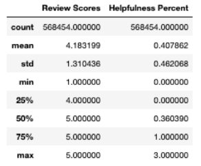
The descriptive statistics of the review scores give us a little more insight, but generally tell us what we already knew: reviews are overwhelmingly positive. The helpfulness percentage, however, is a bit more interesting. The mean helpfulness score is only about 41%, indicating that more often than not, reviewers didn’t find reviews to be helpful. However, this is likely influenced by the high number of reviews that didn’t have any votes. This might indicate that either Amazon shoppers are generally apathetic to reviews of food products and therefore don’t go out of their way to say something when a review was helpful—which may be the case since tastes are so variable—or that the typical Amazon shopper truly didn’t find these reviews very helpful. It might be interesting to compare these findings with reviews of other types of items that aren’t food to see if that makes a difference in engagement with reviews.

9.4 Using Bags for parallel text analysis with NLTK

As we’ve looked at how to transform and filter elements in Bags, something may have become apparent to you: if all the transformation functions are just plain old Python, we should be able to use any Python library that works with generic collections—and that’s precisely what makes Bags so powerful and versatile! In this section, we’ll walk through some typical tasks for preparing and analyzing text data using the popular text analysis library NLTK (Natural Language Toolkit). As motivation for this example, we’ll use the following scenario:

Using NLTK and Dask Bags, find the most commonly mentioned phrases in the text of both positive and negative reviews for Amazon products to see what reviewers frequently discuss in their reviews.

9.4.1 The basics of bigram analysis

To find out more of what the reviewers in this dataset are writing about, we will perform a bigram analysis of the review text. Bigrams are pairs of adjacent words in text. The reason bigrams tend to be more useful than simply counting the frequency of individual words is they typically add more context. For example, we might expect positive reviews to contain the word “good” very frequently, but that doesn’t really help us understand what is good. The bigram “good flavor” or “good packaging” tells us a lot more about what the reviewers find positive about the products. Another thing that we need to do in order to better understand the true subject or sentiment of the reviews is to remove words that don’t help convey that information. Many words in the English language add structure to a sentence but don’t convey information. For example, articles like “the,” “a,” and “an” do not provide any context or information. Because these words are so common (and necessary for proper sentence formation), we’re just as likely to find these words in positive reviews as we are negative reviews. Since they don’t add any information, we will remove them. These are known as stopwords, and one of the most important data preparation tasks when doing text analysis is detecting and removing stopwords. Figure 9.9 shows examples of a few common stopwords.

The process we’ll follow for performing the bigram analysis consists of the following steps:

9.4.2 Extracting tokens and filtering stopwords

Before we jump in, make sure you have NLTK set up properly in your Python environment. See the appendix for instructions on installing and configuring NLTK. With NLTK installed, we need to import the relevant modules into our current workspace; then we’ll create a few functions to help us along with the data prep.

In listing 9.26, we’re defining a few functions to help grab the review text from the original Bag and filter out the stopwords. One thing to point out is the use of the partial function inside the filter_stopwords function. Using partial allows us to freeze the value of the stopwords argument while keeping the value of the word argument dynamic. Since we want to compare every word to the same list of stopwords, the value of the stopwords argument should remain static. With our data preparation functions defined, we’ll now map over the Bag of reviews to extract and clean the review text.

The code in listing 9.27 should be pretty straightforward. We simply use the map function to apply the extracting, tokenizing, and filtering functions to the Bag of reviews. As you can see, we’re left with a Bag of lists, and each list contains all the unique nonstopwords found in the text of each review. If we take one element from this new Bag, we’re returned a list of all words in the first review (except for stopwords, that is). This is important to note: currently our Bag is a nested collection. We’ll come back to that momentarily. However, now that we have the cleaned list of words for each review, we’ll transform our Bag of lists of tokens into a Bag of lists of bigrams.

In listing 9.28, we simply have another function to map over the previously created Bag. Again, this is pretty exciting because this process is completely parallelized using Dask. This means we could use the exact same code to analyze billions or trillions of reviews! As you can see, we now have a list of bigrams. However, we still have the nested data structure. Taking two elements results in two lists of bigrams. We’re going to want to find the most frequent bigrams across the entire Bag, so we need to get rid of the nested structure. This is called flattening a Bag. Flattening removes one level of nesting; for example, a list of two lists containing 5 elements each becomes a single list containing all 10 elements.

After flattening the Bag in listing 9.29, we’re now left with a Bag that contains all bigrams without any nesting by review. It’s now no longer possible to figure out which bigram came from which review, but that’s OK because that’s not important for our analysis. What we want to do is fold this Bag using the bigram as the key, and counting the number of times each bigram appears in the dataset. We can reuse the count and compute functions we defined earlier in the chapter.

The foldby function in listing 9.30 looks exactly like the foldby function you saw earlier in the chapter. However, we’ve chained a new method to it, topk, which gets the top k number of elements when the Bag is sorted in descending order. In the previous example, we get the top 10 elements as denoted by the first parameter of the method. The second parameter, the key parameter, defines what the Bag should be sorted by. The folding function returns a Bag of tuples where the first element is the key and the second element is the frequency. We want to find the top 10 most frequent bigrams, so the Bag should be sorted by the second element of each tuple. Therefore, the key function simply returns the frequency element of each tuple. This has been shortened by using a lambda expression since the key function is so simple. Taking a look at the most common bigrams, it looks like we have some unhelpful entries. For example, “amazon com” is the second most frequent bigram. This makes sense, since the reviews are from Amazon. It looks like some HTML may have also leaked into the reviews, because “br br” is the most common bigram. This is in reference to the HTML tag, <br>, which denotes whitespace. These words aren’t helpful or descriptive at all, so we should add them to our list of stopwords and rerun the bigram analysis.

9.4.3 Analyzing the bigrams

Now that we’ve removed the additional stopwords, we can see some clear topics. For example, “k cups” and “coffee” were mentioned a large number of times. This is probably because many of the reviews are for coffee pods for Keurig coffee machines. The most common bigram is “highly recommend,” which also makes sense because a lot of the reviews were positive. We could continue iterating over our list of stopwords to see what new patterns emerge (perhaps we could remove the words such as “like” and “store” because they don’t add much information), but it would also be interesting to see how the list of bigrams look for reviews that are negative. To close out the chapter, we’ll filter our original set of reviews to those that got only one or two stars, and then see what bigrams are the most common.

The list of bigrams we get from listing 9.32 shares some similarities with the bigrams from all reviews, but also has some distinct bigrams that show frustration or disappointment with the product (“thought would,” “waste money,” and so forth). Interestingly, “taste good” is a bigram for the negative reviews. This might be because reviewers would say something like “I thought it would taste good” or “It didn’t taste good.” This shows that the dataset needs a bit more work—perhaps more stopwords—but now you have all the tools you need to do it! We’ll come back to this dataset in the next chapter, when we’ll use Dask’s machine learning pipelines to build a sentiment classifier that will try to predict whether a review is positive or negative based on its text. In the meantime, hopefully you’ve come to appreciate how powerful and flexible Dask Bags are for unstructured data analysis.

Summary